AI Surrogate Simulation Data

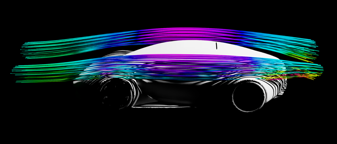
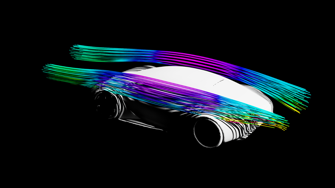
This example visualizes a saved inference result from an automotive external-aerodynamics surrogate. The data is a 128,000-point cloud with velocity, pressure, and turbulence fields stored in a NumPy .npz file.

Kit-CAE uses the same native import, field exploration, and visualization workflow for AI output as it does for solver output.

Dataset

The data is a saved result from the Digital Twins for Fluid Simulation blueprint.

Use the files in:

{path to}/kit_cae_user_guide_data/examples/04_ai-surrogate-simulation-data

File	Field	Description
aero_auto_inference.npz	velocity	Three-component velocity at 128,000 points
aero_auto_inference.npz	pressure	Scalar pressure at 128,000 points
aero_auto_inference.npz	turbulent_kinetic_energy	Scalar turbulent kinetic energy
aero_auto_inference.npz	turbulent_viscosity	Scalar turbulent viscosity
aero_auto_inference.npz	sdf	Signed distance field on a 128 × 64 × 64 grid
aero_auto_low.stl	Geometry	Vehicle surface mesh for spatial context

Note

This example requires the sample data described in Examples. If you have not built Kit-CAE, see Get Started first.

Import the Data

1. Launch Kit-CAE.

   Linux:

   ./repo.sh launch -n omni.cae.kit
   

   Windows:

   repo.bat launch -n omni.cae.kit
   

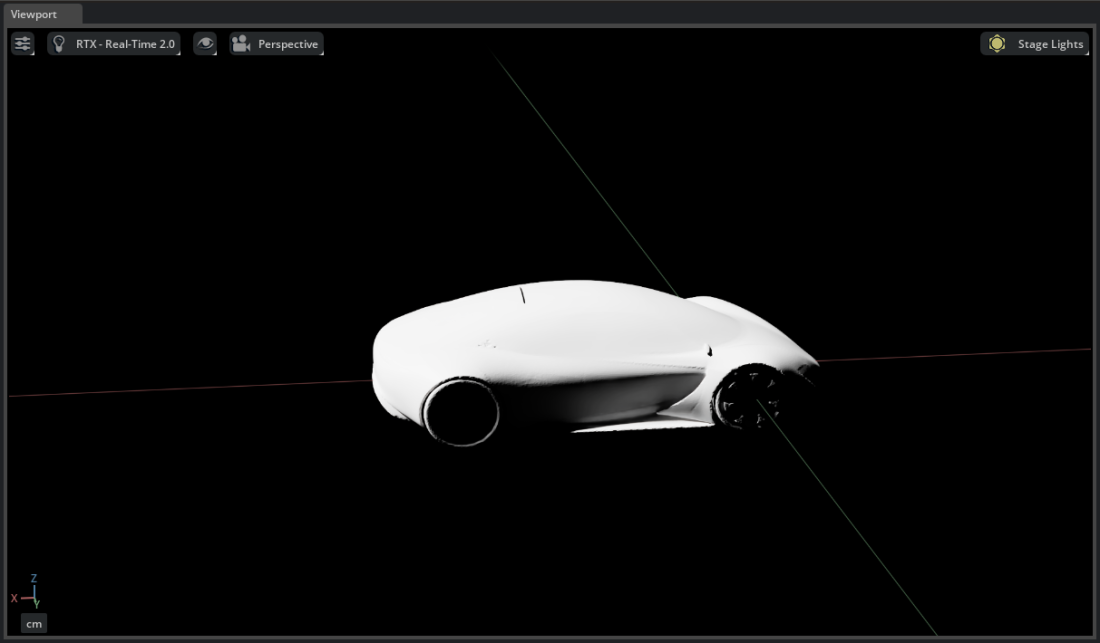
2. Select File > Import, select aero_auto_low.stl, enable Import to Stage, and select Import.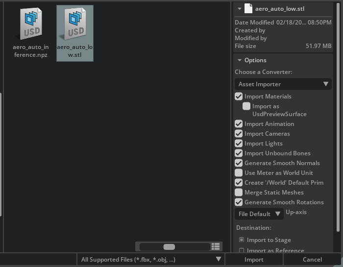

   

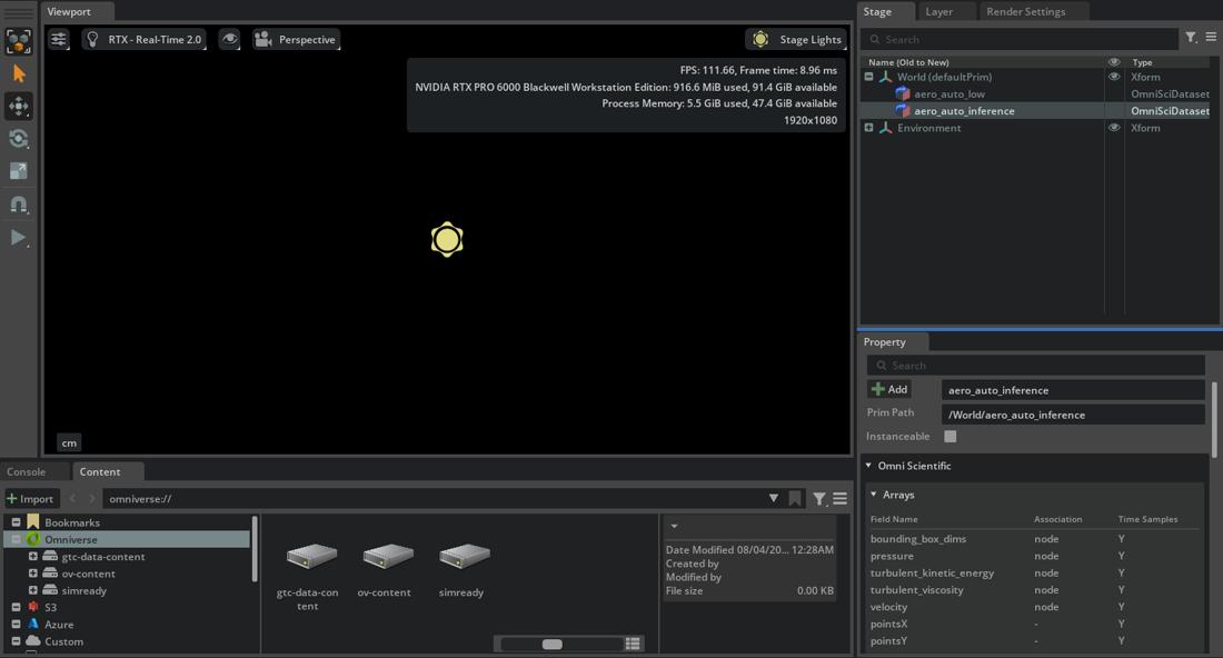
3. Import aero_auto_inference.npz the same way.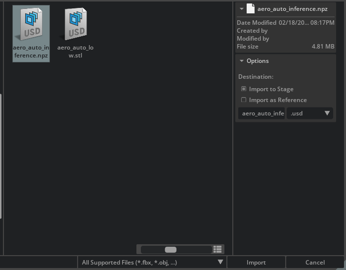

   

NumPy .npz files use the Point Cloud interpretation by default. The STL and point-cloud coordinates already share the same Z-up orientation, so no import-axis adjustment is required for this sample.

Create the Vehicle Surface and Seeds

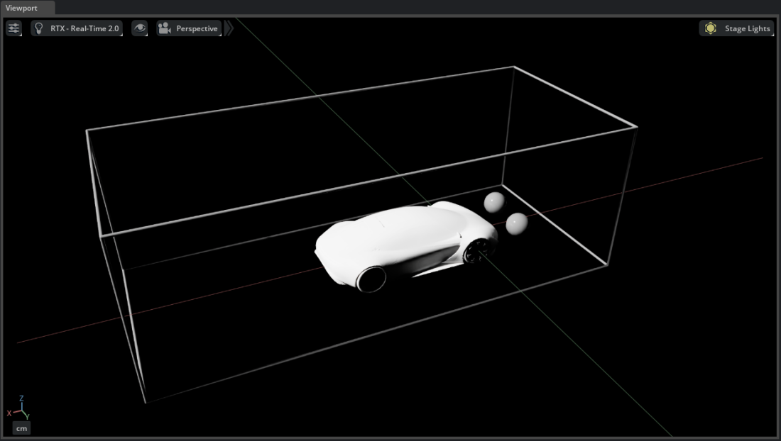
1. Select the imported aero_auto_low dataset and create CAE Operators > Faces.

2. Select aero_auto_inference and create CAE Sources > Bounding Box.

3. Create a Unit Sphere from the Bounding Box with resolution 16.

4. Duplicate the sphere with Ctrl+D.

5. Position the two spheres at different locations in front of the vehicle.

Create Multi-Seed Streamlines

1. Right-click aero_auto_inference and select Create > CAE Operators > Streamlines. Choose nanovdb.

2. Under Source [Gaussian Splatting], set Radius Factor to 4.

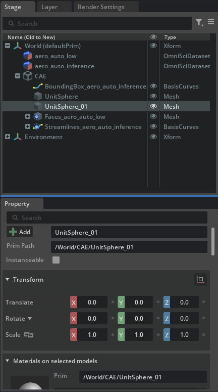
3. Set Direction to forward.

4. Under Seeds [Dataset Selection], select Add Target and choose both Unit Sphere prims.

   

5. Under Velocities [Field Selection], use Add Field to select velocity.

   The velocity array has shape (128000, 3), so one field supplies all three vector components.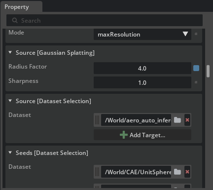

   

6. Under Colors [Field Selection], use Add Field to select velocity and set Mode to vector_magnitude.

7. Set the colors Rescale Mode to disable. On Materials > ScalarColor > Shader, start with a domain of 20 through 35 and adjust it for the features of interest.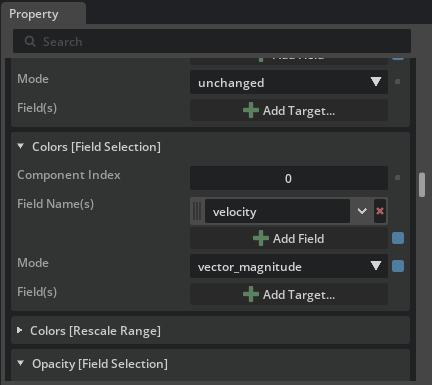

   

Move either Unit Sphere to compare flow paths from another seed region. The source remains the saved NumPy inference result throughout the workflow; no conversion to a solver format is required.

Explore Other Fields

Select the imported aero_auto_inference dataset. In Arrays, select pressure, turbulent_kinetic_energy, or turbulent_viscosity, then use Array Details > Compute Details to choose a meaningful range for another visualization.

Return to velocity and the fixed 20 through 35 color domain to finish with the multi-seed streamline result.