Create Operators

Operators are dynamic visualization entities. To create one, right-click a prim in the Stage panel and navigate to Create > CAE Operators. They re-execute on stage reload, generating results on-the-fly from the source data. Each operator prim has the Omni CAE Operator API applied.

Common Operator Properties

All operators share these properties in the Properties panel under the CAE group:

• Compute Device: auto uses the global preference, or override per-operator to a specific device (CPU, CUDA).

• Enabled: Toggle to disable execution. Useful for debugging, performance tuning, or configuring the full pipeline before any operator runs.

• Source: The dataset the operator reads from. Set automatically based on which node you right-clicked when creating the operator.

Faces

The Faces operator extracts and renders the boundary surfaces of a volumetric mesh. Use it when you want to see the shape of your simulation domain or color the outer skin of a mesh by a field value like pressure or wall shear stress.

1. In the Stage panel, right-click on a dataset node.

2. Navigate to Create > CAE Operators > Faces.

The operator creates a surface mesh from the outer faces of the volume. To color by a scalar field, use the field selection property to choose a field and, for vector fields, a specific component or magnitude.

Note

For polyhedral datasets, apply the Faces operator to the surface mesh blocks in the stage tree rather than the volumetric mesh block. Extracting interior faces from polyhedral volumes is not yet supported.

Points

The Points operator renders a sphere at every vertex in the dataset. Use it for a quick structural overview of your data: seeing where the mesh nodes are, how dense the resolution is, or visualizing point cloud data that has no mesh connectivity.

1. Right-click on a dataset node and select Create > CAE Operators > Points.

2. In the operator’s properties, adjust the Width value to control sphere size (for example, 0.05).

To color the points by a scalar quantity, use the field selection property to choose a field from the dataset. To vary point size by a data value, use the Widths field selection.

Note

For datasets with mesh connectivity, Faces is usually a better choice because it shows the actual surface geometry. Use Points when you need a lightweight representation, when working with point clouds (for example, NumPy or particle data), or when you want to inspect individual node locations.

Glyphs

The Glyphs operator places oriented 3D shapes at data point locations. Use it to visualize vector fields, for example arrows showing velocity direction and magnitude across a flow domain, or to represent any quantity where direction and scale matter.

1. Right-click on a dataset node and select Create > CAE Operators > Glyphs.

2. Choose a glyph shape:

   • Arrow: Best for vector field visualization (velocity, force direction).

   • Cone: Directional indicator without an explicit head or tail.

   • Sphere: Uniform shape, useful when only position and size matter.

3. In the operator’s properties:

   • Next to Orientations, click Add Target and select the vector field components that define glyph direction (for example, the three velocity components).

   • Next to Scales, click Add Target and select a field to vary glyph size by data value.

   • Next to Colors, click Add Target and select a field for coloring.

Key Properties:

• Max Count: Maximum number of glyphs to render (default: 10,000,000). Set to 0 to show all points.

• Use Cell Points: When enabled, only places glyphs at points belonging to mesh cells, excluding isolated nodes.

• Orientations Mode: How to interpret the orientation field. eulerAngles (default) treats three components as directional angles. quaternion expects four-component rotation values.

Without any fields attached, all glyphs render at uniform size and orientation. Add field selections incrementally to build up the visualization.

Streamlines

The Streamlines operator traces particle paths through a vector field, showing how fluid flows through the domain. It requires a seed source (where streamlines originate) and a velocity field (which drives the integration). Use it to understand flow patterns, recirculation zones, or wake structures.

1. Create a Unit Sphere source (see Create Sources) and position it in the region of interest.

2. Right-click on a volumetric dataset node and select Create > CAE Operators > Streamlines.

3. In the operator’s properties:

   • Next to Seeds, click Add Target and select the Unit Sphere.

   • Next to Velocity, click Add Target and select the velocity field from the dataset.

4. Move the Unit Sphere to update the streamline positions interactively.

Key Properties:

• dx: Step size between streamline vertices

• Max Length: Maximum distance streamlines are traced

• Width: Display width of the streamlines

• Region of Interest: Limit streamlines to a spatial subset (use a bounding box source)

For NanoVDB-based streamlines, voxelization properties also apply (see Voxelization Properties below).

Volume

The Volume operator renders volumetric data using NVIDIA IndeX.

1. Right-click on a volumetric dataset node and select Create > CAE Operators > Volume.

2. Choose the rendering approach:

   • NanoVDB (default): Recommended for large datasets. Voxelizes the data first.

   • Irregular: Renders the unstructured mesh directly without voxelization.

Note

NanoVDB voxelizes the data onto a regular grid and renders on the GPU. It is faster and recommended for most datasets. Irregular renders the native unstructured mesh directly on the CPU, preserving original cell topology. Use it when voxelization would lose important detail, such as thin boundary layers or sharp gradients near walls. Irregular mode requires that all faces in the mesh are triangles or quadrilaterals; datasets with polyhedral faces must use NanoVDB.

1. In the operator’s properties, select Add Target next to Field and choose the field to visualize.

2. Optionally set a Region of Interest to subset the domain.

The colormap is configured via the operator’s Material/Colormap prim in the Stage panel. Use the interactive gradient adjuster in the Properties panel to control color and translucency (the transfer function).

For volume rendering of point cloud data without mesh connectivity, see AI Surrogate Simulation Data.

Slice

The Slice operator creates a planar cross-section through the dataset.

1. Right-click on a dataset node and select Create > CAE Operators > Slice.

2. In the operator’s properties, select Add Target next to Field and choose the field to display on the slice.

3. Expand the operator in the Stage panel to access the Plane prim. Use the transform gizmo to translate and rotate the plane to the desired position.

4. Duplicate the plane and reposition it for additional slices (optional).

To create two or three orthogonal planes in a single step, select Biplane or Triplane when creating the Slice. This is useful for inspecting a volume from all three principal directions simultaneously.

Note

The initial placement of the slice plane may be outside the visible region. Press F to fit the view and use the transform gizmo to move the plane into the data.

Voxelization Properties

These properties apply to operators that use NanoVDB data (Volume and NanoVDB Streamlines). They are stored directly on the operator prim, not in local preferences. This means the same stage always produces the same voxelization result, even when shared between users or reopened later.

• Max Resolution: Cell count along the longest axis. The voxelization uses uniform voxel spacing. This is the recommended default because it does not require knowledge of the exact data bounds.

• Voxel Size: An explicit voxel size alternative. Use this only if you know your data bounds and need precise control.

• Region of Interest: Subset the domain before voxelizing. Select a bounding box source to limit the voxelized region.

• Explode Bounds: Expand the voxelization region beyond the selected bounds.

Try It: Visualize the Vehicle Dataset

In the previous Try It you created a bounding box and a Unit Sphere on the vehicle dataset. Now use them with operators. You will adjust colors and ranges on these operators in the next section.

Faces

Create surface representations of the vehicle body and wheels.

1. In the Stage panel, hold Shift or Ctrl and select all three surface prims:

   • /World/auto_aero_solver_result/auto_aero_solver_result_cgns/Base/Fluid_Domain/body_Surface

   • /World/auto_aero_solver_result/auto_aero_solver_result_cgns/Base/Fluid_Domain/front_wheels_Surface

   • /World/auto_aero_solver_result/auto_aero_solver_result_cgns/Base/Fluid_Domain/rear_wheels_Surface

2. Right-click and select Create > CAE Operators > Faces.

   

   Three new Faces prims appear under /World/CAE/. The vehicle body and wheels are now visible in the viewport.

   

Streamlines

1. Select /World/auto_aero_solver_result/auto_aero_solver_result_cgns/Base/Fluid_Domain/Fluid_Domain, right-click, and select Create > CAE Operators > Streamlines.

2. When prompted to select a streamlines type, choose NanoVDB.

   

   Nothing appears in the viewport yet. The streamlines operator needs a seed source and velocity field before it can compute.

3. Select /World/CAE/Streamlines_Fluid_Domain in the Stage panel. In the Property panel, scroll to the Streamlines section and set Direction to Forward.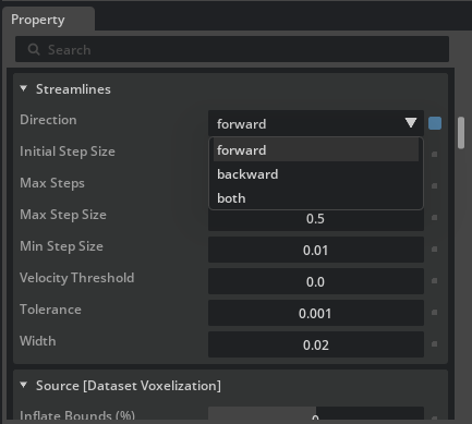

   

4. Scroll to Seeds [Dataset Selection] and click Add Target. Select /World/CAE/UnitSphere.

   

5. Scroll to Velocities [Field Selection] and click Add Target. In the popup, shift-select all three velocity components:

   • /World/auto_aero_solver_result/auto_aero_solver_result_cgns/Base/Fluid_Domain/FlowSolution/Velocity_0

   • /World/auto_aero_solver_result/auto_aero_solver_result_cgns/Base/Fluid_Domain/FlowSolution/Velocity_1

   • /World/auto_aero_solver_result/auto_aero_solver_result_cgns/Base/Fluid_Domain/FlowSolution/Velocity_2

   

   Streamlines appear in the viewport, tracing flow paths from the sphere through the volume.

   

Tip

Select the UnitSphere in the Stage panel and use the transform gizmo to move it around the domain. The streamlines update to show flow paths from the new position. This is a quick way to explore the flow field interactively.

Volume

1. Select /World/auto_aero_solver_result/auto_aero_solver_result_cgns/Base/Fluid_Domain/Fluid_Domain, right-click, and select Create > CAE Operators > Volume. Choose NanoVDB.

2. Select /World/CAE/Volume_Fluid_Domain in the Stage panel. In the Property panel, scroll to the Source [Dataset Voxelization] section, set Max Resolution to 512 within voxelization settings.

   

3. Scroll to Colors [Field Selection] and click Add Target. Shift-select Velocity_0, Velocity_1, and Velocity_2 from FlowSolution. You will adjust the color range in the next section.

   

   Note: The bounding box appears uniformly filled because no color thresholding has been applied yet. You will adjust the color range and transfer function in the next section to reveal the flow structure within the volume.

Slice

1. Right-click /World/CAE/Volume_Fluid_Domain and select Create > CAE Sources > Volume Slice.

   A slice plane appears in the viewport. You will position and configure it in the next section.

   

   Note: The slice plane is now visible inside the volume bounding box. Like the volume, it appears uniform because coloring and thresholding have not been configured yet.

At this point the visualization may look rough; colors and scales are default or have not been selected. The next section covers how to set color fields, adjust ranges, and configure colormaps to produce clearer results.

Tip

You can show or hide any operator or source by clicking the eye icon next to its prim in the Stage panel. This is useful for isolating individual results as you build up the visualization.