Simulation Data in Context

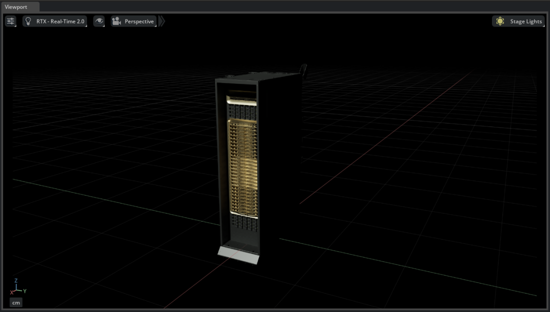
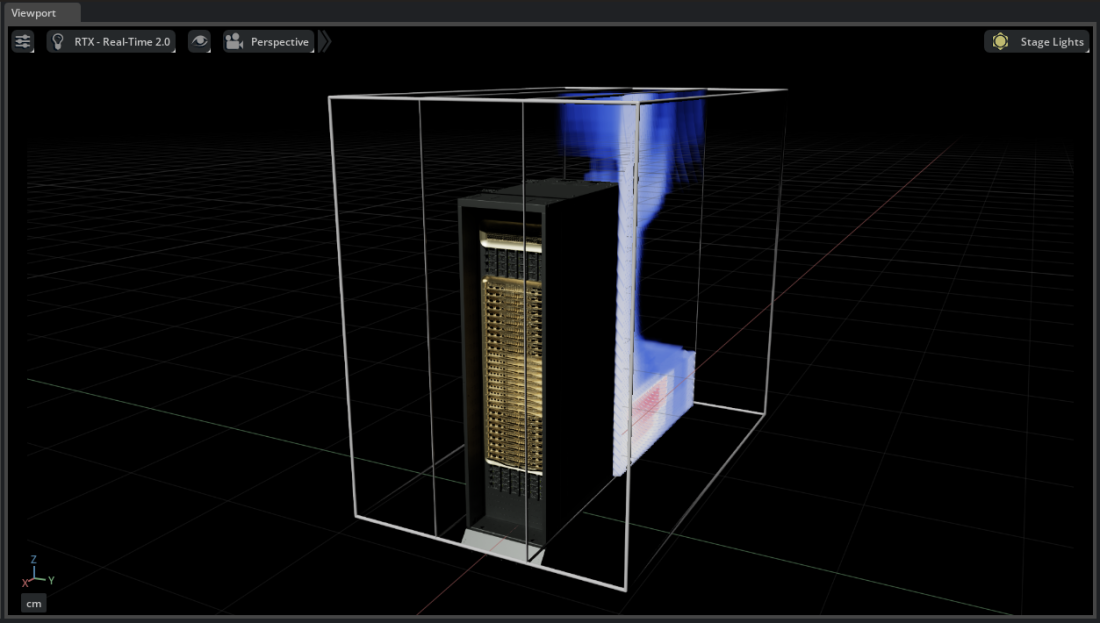
Simulation results are most meaningful when viewed alongside the geometry they describe. This example overlays a steady-state thermal simulation onto a full-fidelity NVIDIA GB300 NVL72 server rack, showing hot-aisle air temperature during operation. The thermal data (CGNS) and the rack geometry (USD) come from different sources; Kit-CAE composes them into a single scene via OpenUSD without converting either.

This example uses simplified thermal data inspired by the type of analysis performed in the NVIDIA Omniverse Blueprint for AI Factory Digital Twins. The thermal field was extracted from a larger computed domain, so the influence of surrounding racks and other infrastructure is present in the results. Here we view only the region near a single GB300.

Note

This example requires sample data. If you have not already downloaded it, see Examples for the download link.

Dataset

The sample data contains a steady-state thermal simulation result and a detailed rack model. Both are subsets of the larger AI factory digital twin; the thermal field covers the volume around a single rack.

File	Format	Field	Description
compute_thermal.cgns	CGNS	Temperature	Steady-state air temperature near the rack (cell-centered, C)
GB300.usd	USD	(geometry)	Full-fidelity GB300 NVL72 server rack model

• Mesh: ~71,500 nodes, ~57,100 hexahedral elements

• Time: Steady-state (single snapshot)

Import the Data

Note

This walkthrough assumes you have already built Kit-CAE. If not, see Get Started for setup instructions.

1. Launch Kit-CAE.

   On Linux:

   ./repo.sh launch -n omni.cae.kit
   

   On Windows:

   repo.bat launch -n omni.cae.kit
   

2. Click File > Open and navigate to:

   {path to}/kit_cae_user_guide_data/examples/02_simulation-data-in-context/GB300.usd

   The GB300 rack model loads and appears in the viewport.

   

3. Click File > Import and navigate to:

   {path to}/kit_cae_user_guide_data/examples/02_simulation-data-in-context/compute_thermal.cgns

   Check Import to Stage and click Import. A new compute_thermal prim appears in the Stage panel. Nothing new is visible in the viewport yet.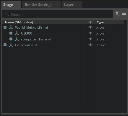

   

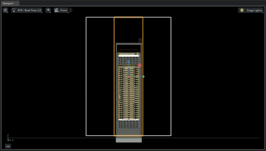
Create Bounding Boxes

Next, create two bounding boxes. The first covers the full extent of the thermal data. The second is scaled to focus on the region directly behind the rack; this narrower box will serve as a Region of Interest (ROI) for the volume operator.

Remember that sources are simple USD prims. Once created, they are not linked to the imported data. You can duplicate, rename, scale, and reposition them freely.

1. In the Stage panel, expand the thermal dataset to /World/compute_thermal/compute_thermal_cgns/Base/Zone/Elements. Right-click Elements and select Create > CAE Sources > Bounding Box.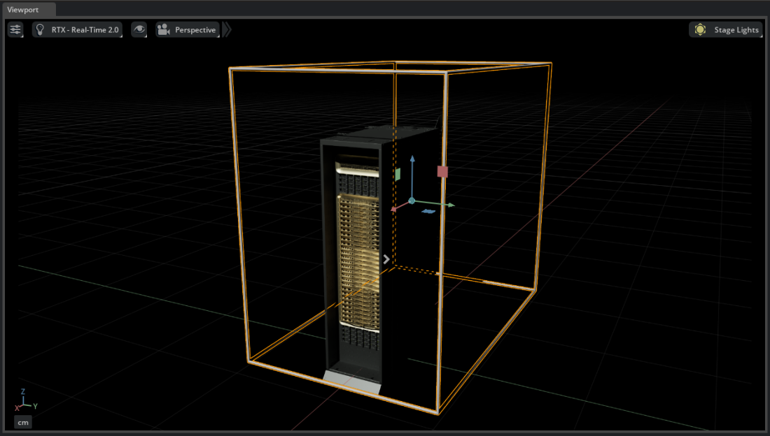

   

2. Select the bounding box you just created. Press Ctrl+D to duplicate it.

3. With the duplicate selected, press R to switch to the scale gizmo. Scale it to more closely fit the rack, focusing on the hot-aisle region directly behind the GB300. Press W to return to the translate gizmo when done.

Create a Volume Operator

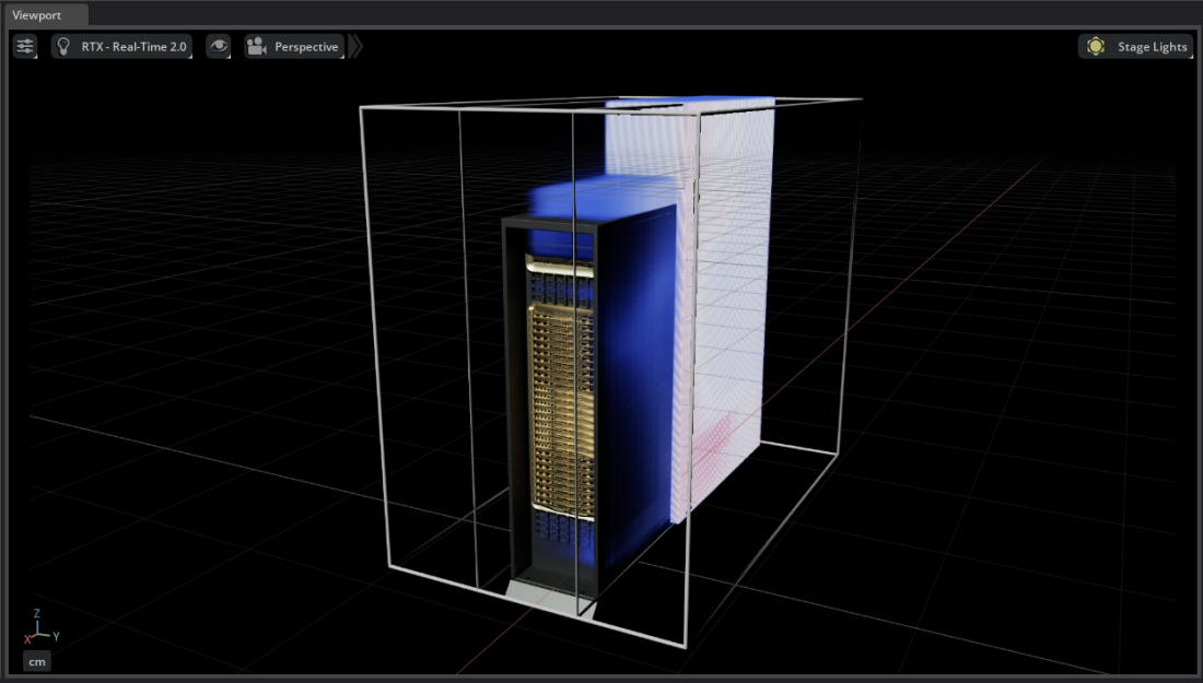
1. Right-click Elements and select Create > CAE Operators > Volume.

2. When prompted, choose NanoVDB.

   

Note

The Irregular option works directly on the unstructured mesh without voxelization. It preserves exact cell geometry and is useful when accuracy matters more than speed (for example, validation or detailed analysis near boundaries). NanoVDB first resamples the data onto a sparse voxel grid, then renders on the GPU; this is faster for interactive exploration but trades sub-voxel detail for performance.

This dataset uses only triangular and quadrilateral faces, which means Irregular mode is available here. Many of the datasets in the main guide use polyhedral elements that require NanoVDB. If you want to try Irregular mode on this data, select it instead; note that it will take longer to compute. This walkthrough continues with NanoVDB.

Visualize the Thermal Field

1. Select the Volume operator prim in the Stage panel. In the Property panel, scroll to Region-of-interest (ROI) and click Add Target. Select the narrower bounding box you created.

   

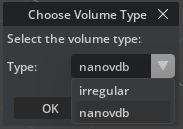
2. Scroll to Colors [Field Selection] and click Add Target. Navigate to /World/compute_thermal/compute_thermal_cgns/Base/Zone/SolutionCellCenter/Temperature and click Select.

   The thermal field appears in the viewport, overlaid on the rack geometry.

   

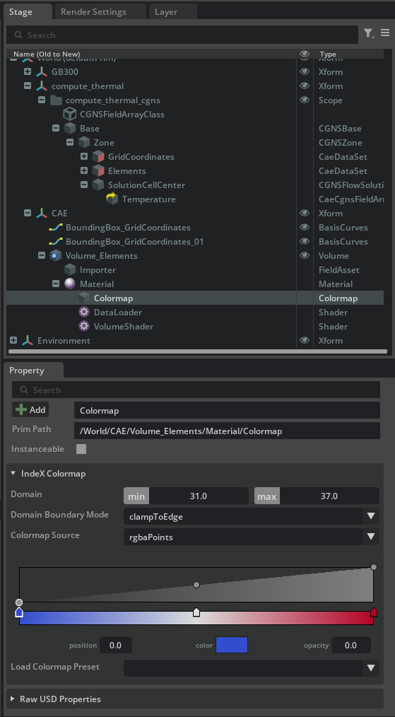
3. Expand the Volume operator in the Stage panel and navigate to Material > Colormap. Adjust the color range and transfer function to better reveal the temperature gradients near the rack.

   

Tip

Toggle the rack visibility (eye icon on the GB300 prim) to see the thermal field alone, then re-enable it to view the results in context with the geometry.