AI Surrogate Simulation Data

This example visualizes a saved inference result from an automotive external aerodynamics surrogate. The data is a 128,000-point cloud with velocity, pressure, and turbulence fields stored as a NumPy .npz file.

Inference data from a surrogate model is treated the same as solver output. The same import path, the same visualization operators, and the same algorithms apply. OpenUSD serves as the composition and access layer regardless of where the data originated.

Note

This example requires sample data. If you have not already downloaded it, see Examples for the download link.

Dataset

The data is a saved inference result from the Digital Twins for Fluid Simulation blueprint, which uses an automotive external aerodynamics surrogate model.

File	Format	Field	Description
aero_auto_inference.npz	NumPy	velocity	3-component velocity at 128,000 points
aero_auto_inference.npz	NumPy	pressure	Scalar pressure at 128,000 points
aero_auto_inference.npz	NumPy	turbulent_kinetic_energy	Scalar TKE at 128,000 points
aero_auto_inference.npz	NumPy	turbulent_viscosity	Scalar turbulent viscosity at 128,000 points
aero_auto_inference.npz	NumPy	sdf	Signed distance field (128 x 64 x 64 volumetric grid)
aero_auto_low.stl	STL		Vehicle surface mesh (reference geometry for spatial context)

• Time: single snapshot

Import the Data

Note

This walkthrough assumes you have already built Kit-CAE. If not, see Get Started for setup instructions.

1. Launch Kit-CAE.

   On Linux:

   ./repo.sh launch -n omni.cae.kit
   

   On Windows:

   repo.bat launch -n omni.cae.kit
   

2. Click File > Import and navigate to:

   {path to}/kit_cae_user_guide_data/examples/04_ai-surrogate-simulation-data

3. Select aero_auto_low.stl. In the import options, set Up Axis to Z. Check Import to Stage and click Import. This is the vehicle surface mesh; it provides spatial context for the simulation data.

   

4. Press F to focus the viewport on the imported geometry.

5. Click File > Import again and select aero_auto_inference.npz from the same folder. In the import options, select Point Cloud. Check Import to Stage and click Import.

   

   After both imports, the vehicle mesh is visible in the viewport and both prims appear in the Stage panel.

Create Sources

1. In the Stage panel, expand the point cloud dataset to /World/aero_auto_inference/aero_auto_inference_npz/NumPyDataSet. Right-click NumPyDataSet and select Create > CAE Sources > Bounding Box.

2. With the bounding box selected, right-click and select Create > CAE Sources > Unit Sphere. This creates the first seed source.

3. Select the UnitSphere you just created and press Ctrl+D to duplicate it. This creates a second seed source.

   Remember that sources are simple USD prims. Once created, they are not linked to the imported data. You can duplicate, rename, scale, and reposition them freely.

4. Position the two spheres at different locations in front of or around the vehicle. Having multiple seeds lets you trace streamlines from several regions simultaneously.

   

Multi-Seed Streamlines

This example demonstrates multi-seed streamlines: a single Streamlines operator with more than one seed source. This is useful for comparing flow behavior from multiple starting regions without creating separate operators.

1. Select /World/aero_auto_inference/aero_auto_inference_npz/NumPyDataSet, right-click, and select Create > CAE Operators > Streamlines. Choose NanoVDB.

2. Select the Streamlines prim in the Stage panel. In the Property panel, scroll to the Source [Gaussian Splatting] section and set Radius Factor to 4.

3. Scroll to the Streamlines section and set Direction to Forward.

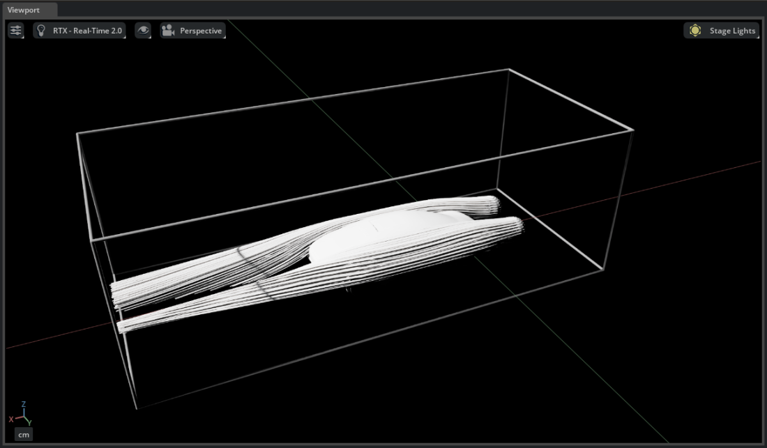
4. Scroll to Seeds [Dataset Selection] and click Add Target. In the popup, shift-select or ctrl-select /World/CAE/UnitSphere and /World/CAE/UnitSphere_01 and click Select.

   Both seeds appear in the Seeds section. The streamlines operator traces paths from every vertex on both spheres.

   

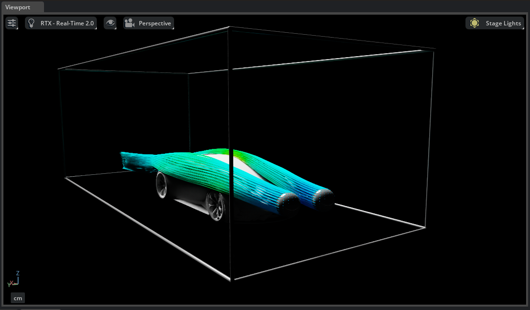
5. Scroll to Velocities [Field Selection] and click Add Target. Select the velocity field from the dataset. Unlike the main guide where velocity was stored as three separate single-component fields (requiring multi-select), this dataset stores all three components in a single field (shape N,3). A single selection is sufficient.

   Streamlines appear in the viewport, tracing flow paths from both seed locations through the point cloud data.

   

6. Scroll to Colors [Field Selection] and click Add Target. Select the velocity field to color by velocity magnitude, or select pressure for pressure coloring.

7. Expand the Streamlines prim in the Stage panel and navigate to Materials > ScalarColor > Shader. Adjust the domain fields to set a meaningful color range. Lock the domain to keep it fixed when moving the seeds.

   

Tip

Select one or both UnitSphere prims and move them to new positions. The streamlines update from the new locations, letting you compare flow behavior from different regions side by side.