Rigid Bodies#
Rigid bodies are used to represent objects that can move without deforming. Their motion is typically affected by external forces such as gravity, collisions with other objects (if associated with colliders), and other constraints, such as joints. When configured as kinematic, their motion can be fully controlled by the application to influence other objects.
A rigid body is represented in the USD stage hierarchy as a prim of type UsdGeom.Xformable with the applied UsdPhysics.RigidBodyAPI. The prim with UsdPhysics.RigidBodyAPI and all of its descendant prims move as one rigid object.
If, for some reason, a given USD stage hierarchy is unsuitable for representing the required rigid bodies with their sub-trees, the hierarchy can be broken up using the resetXformStack attribute of the UsdGeom.Xformable type. For example, if the resetXformStack attribute is set on a rigid body prim, its transform is decoupled from its parent. This makes it possible to nest rigid bodies in the stage hierarchy, which is otherwise invalid.
Create and Destroy a Rigid Body#
A rigid body may be created by applying UsdPhysics.RigidBodyAPI to a prim of type UsdGeom.Xformable. The following Python snippet demonstrates the creation and destruction of a rigid body:
from pxr import Usd, UsdGeom, UsdPhysics, Gf
import omni.usd

# Create a stage
omni.usd.get_context().new_stage()
stage = omni.usd.get_context().get_stage()

# Define the root Xform (transformable object)
rootxform = UsdGeom.Xform.Define(stage, "/World")

# Create an xformable
rigidBodyPath = "/World/rigidBody"
rigidBodyXform = UsdGeom.Xform.Define(stage, rigidBodyPath)
rigidBodyPrim = rigidBodyXform.GetPrim()

# Apply RigidBodyAPI to the xformable
rigidBodyAPI = UsdPhysics.RigidBodyAPI.Apply(rigidBodyPrim)

# Remove the rigid body
stage.RemovePrim(rigidBodyPath)
Kinematic Rigid Body#
Rigid bodies can be configured in two ways:
By default rigid bodies are created as dynamic objects that are moved by the simulation. Their velocity is the product of forces and constraints integrated over time.
Alternatively rigid bodies can be configured to act as kinematic objects, in which case their motion is directly controlled by the application.
Another way to think about dynamic vs. kinematic rigid bodies is in terms of transform read/write access by the simulation engine:
a dynamic rigid body has its transform written to by the simulation.
a kinematic rigid body’s transform is read by the simulation.
The following code snippet demonstrates how a rigid body can be created and, optionally, configured as kinematic object:
from pxr import Usd, UsdGeom, UsdPhysics, Gf
import omni.usd

# Create a stage
omni.usd.get_context().new_stage()
stage  = omni.usd.get_context().get_stage()

# Define the root Xform (transformable object)
rootxform = UsdGeom.Xform.Define(stage, "/World")

rigidBodyPaths = ["/World/rigidBody0", "/World/rigidBody1"]
enableKinematic = [False, True]

for i in range(2):
    rigidBodyXform = UsdGeom.Xform.Define(stage, rigidBodyPaths[i])
    rigidBodyPrim = rigidBodyXform.GetPrim()
    rigidBodyAPI = UsdPhysics.RigidBodyAPI.Apply(rigidBodyPrim)
    if enableKinematic[i]:
        rigidBodyAPI.CreateKinematicEnabledAttr(True)
    isKinematic = rigidBodyAPI.GetKinematicEnabledAttr().Get()
    print(f"i = {i}: Kinematic enabled is {isKinematic}")
Disabling a Rigid Body#
All prims in the sub-tree of a rigid body prim translate and rotate rigidly with the motion of the rigid body, following the rules of the transform hierarchy. This includes colliders on or below the rigid body prim. Disabling a rigid body by setting its rigidBodyEnabled attribute to False cancels any effect of the UsdPhysics.RigidBodyAPI. As a result any colliders in the sub-tree act as static colliders.
The following Python script demonstrates how a rigid body can be created and then disabled:
from pxr import Usd, UsdGeom, UsdPhysics, Gf
import omni.usd

# Create a stage
omni.usd.get_context().new_stage()
stage  = omni.usd.get_context().get_stage()

# Define the root Xform (transformable object)
rootxform = UsdGeom.Xform.Define(stage, "/World")

rigidBodyPath = "/World/rigidBody"

rigidBodyXform = UsdGeom.Xform.Define(stage, rigidBodyPath)
rigidBodyPrim = rigidBodyXform.GetPrim()
rigidBodyAPI = UsdPhysics.RigidBodyAPI.Apply(rigidBodyPrim)
rigidBodyAPI.GetRigidBodyEnabledAttr().Set(False)
Rigid Body Frames#
Rigid body setups have multiple associated coordinate frames. These are referred to here as:
rigid-body-prim frame
center of mass frame (see section Configure Rigid Body Mass Properties)
collider frames (see section Create a Rigid Body with a Collider)
joint local frames (see section Joint Frames)
velocity frames (see section Set Rigid Body Velocity)
force frames (see section Apply Force to a Rigid Body)
The rigid body may be considered as a container of sub-frames. Internally, simulation proceeds with reference to the center of mass. The introduction of the concept of the rigid-body-prim frame, however, provides a common reference for joints and colliders. This allows, for example, the center of mass to be modified without impacting joint or collider frames defined relatively to the rigid-body-prim frame.
The rigid-body-prim frame describes the pose of the prim with the UsdPhysics.RigidBodyAPI relative to the origin of the world coordinate frame. The center of mass frame, on the other hand, is specified relative to the rigid body frame. The position and orientation of the center of mass frame in the world coordinate frame is therefore a function of the rigid body pose in the world frame and the center of mass pose in the rigid body frame. Collider and joint local frames are similarly specified in the frame of an associated rigid body.
Create a Rigid Body with a Collider#
This section introduces the creation of rigid bodies with colliders, which allows them to collide with other objects in the scene.
Static colliders are discussed in section Create and Destroy a Static Collider.
Collider prims are associated with rigid body prims by their relative location in the USD stage hierarchy. A collider in the sub-tree of a rigid body prim is part of that rigid body and can be posed relative to the rigid body transformation frame employing the USD transformation hierarchy.
The following Python script illustrates the creation of a rigid body with cube collision geometry:
from pxr import Usd, UsdGeom, UsdPhysics, Gf
import omni.usd

# Create a stage
omni.usd.get_context().new_stage()
stage  = omni.usd.get_context().get_stage()

# Define the root Xform (transformable object)
rootxform = UsdGeom.Xform.Define(stage, "/World")

rigidBodyPath = "/World/rigidBody"
cubePath = rigidBodyPath + "/cube"

# Properties of the geometry
cubePosition = Gf.Vec3f(2.0, 0.0, 0.0)
cubeOrientation = Gf.Quatf(1.0)
cubeScale = Gf.Vec3f(1.0, 1.0, 1.0)
cubeSize = 2.0
cubeHalfExtent = cubeSize/2.0

# Create a rigid body
rigidBodyXform = UsdGeom.Xform.Define(stage, rigidBodyPath)
rigidBodyXform.AddTranslateOp().Set(Gf.Vec3f(0.0))
rigidBodyXform.AddOrientOp().Set(Gf.Quatf(1.0))
rigidBodyPrim = rigidBodyXform.GetPrim()
UsdPhysics.RigidBodyAPI.Apply(rigidBodyPrim)

# Create the cube as a child of the rigid body prim
cubeGeom = UsdGeom.Cube.Define(stage, cubePath)
cubeGeom.CreateSizeAttr(cubeSize)
cubeGeom.CreateExtentAttr([Gf.Vec3f(-cubeHalfExtent), Gf.Vec3f(cubeHalfExtent)])
cubeGeom.AddTranslateOp().Set(cubePosition)
cubeGeom.AddOrientOp().Set(cubeOrientation)
cubeGeom.AddScaleOp().Set(cubeScale)
cubePrim = cubeGeom.GetPrim()
UsdPhysics.CollisionAPI.Apply(cubePrim)
The cube collider in the snippet is created as a child of the rigid body. As a result, the pose assigned to the collider prim is represented relative to the rigid body frame, as discussed in section Rigid Body Frames.
Configure a Rigid Body with multiple Colliders#
The previous script example can be extended to create a rigid body with multiple colliders. The following script demonstrates a rigid body with two cube colliders, each centered at a different position relative to the parent:
from pxr import Usd, UsdGeom, UsdPhysics, Gf
import omni.usd

# Create a stage
omni.usd.get_context().new_stage()
stage  = omni.usd.get_context().get_stage()

# Define the root Xform (transformable object)
rootxform = UsdGeom.Xform.Define(stage, "/World")

rigidBodyPath = "/World/rigidBody"
cubePaths = [rigidBodyPath + "/cube0", rigidBodyPath + "/cube1"]
cubePositions = [Gf.Vec3f(-2.0, 0.0, 0.0), Gf.Vec3f(2.0, 0.0, 0.0)]
cubeOrientation = Gf.Quatf(1.0)
cubeScale = Gf.Vec3f(1.0, 1.0, 1.0)
cubeSize = 2.0
cubeHalfExtent = cubeSize/2.0

# Create the rigid body
rigidBody = UsdGeom.Xform.Define(stage, rigidBodyPath)
rigidBody.AddTranslateOp().Set(Gf.Vec3f(0.0))
rigidBody.AddOrientOp().Set(Gf.Quatf(1.0))
rigidBodyPrim = rigidBody.GetPrim()
UsdPhysics.RigidBodyAPI.Apply(rigidBodyPrim)

for i in range(2):

    # Create the cube as a child of the rigid body prim
    cubeGeom = UsdGeom.Cube.Define(stage, cubePaths[i])
    cubeGeom.CreateSizeAttr(cubeSize)
    cubeGeom.CreateExtentAttr([Gf.Vec3f(-cubeHalfExtent), Gf.Vec3f(cubeHalfExtent)])
    cubeGeom.AddTranslateOp().Set(cubePositions[i])
    cubeGeom.AddOrientOp().Set(cubeOrientation)
    cubeGeom.AddScaleOp().Set(cubeScale)
    cubePrim = cubeGeom.GetPrim()
    UsdPhysics.CollisionAPI.Apply(cubePrim)
In the above example, cube0 is positioned at (-2, 0, 0), while cube1 is positioned at (2, 0, 0)
Configure Rigid Body’s Material Properties#
UsdPhysics.MaterialAPI can be used to create physics material properties (static friction, dynamic friction, restitution, and density) when applied to a material prim. The density attribute is discussed in more detail in section Automatic Computation of Rigid Body Mass Distribution.
The following snippet illustrates binding a material to a rigid actor using UsdShade.MaterialBindingAPI with a “physics” purpose:
from pxr import Usd, UsdGeom, UsdShade, UsdPhysics, Gf, PhysxSchema
import omni.usd

# Create a stage
omni.usd.get_context().new_stage()
stage  = omni.usd.get_context().get_stage()

# Define the root Xform (transformable object)
rootxform = UsdGeom.Xform.Define(stage, "/World")

rigidBodyPath = "/World/rigidBody"
cubePath = rigidBodyPath + "/cube"
materialPath = "/path/to/material"

# Properties of the geometry
cubePosition = Gf.Vec3f(2.0, 0.0, 0.0)
cubeOrientation = Gf.Quatf(1.0)
cubeScale = Gf.Vec3f(1.0, 1.0, 1.0)
cubeSize = 2.0
cubeHalfExtent = cubeSize/2.0

# Create a rigid body
rigidBodyXform = UsdGeom.Xform.Define(stage, rigidBodyPath)
rigidBodyXform.AddTranslateOp().Set(Gf.Vec3f(0.0))
rigidBodyXform.AddOrientOp().Set(Gf.Quatf(1.0))
rigidBodyPrim = rigidBodyXform.GetPrim()
UsdPhysics.RigidBodyAPI.Apply(rigidBodyPrim)

# Create the cube as a child of the rigid body prim
cubeGeom = UsdGeom.Cube.Define(stage, cubePath)
cubeGeom.CreateSizeAttr(cubeSize)
cubeGeom.CreateExtentAttr([Gf.Vec3f(-cubeHalfExtent), Gf.Vec3f(cubeHalfExtent)])
cubeGeom.AddTranslateOp().Set(cubePosition)
cubeGeom.AddOrientOp().Set(cubeOrientation)
cubeGeom.AddScaleOp().Set(cubeScale)
cubePrim = cubeGeom.GetPrim()
UsdPhysics.CollisionAPI.Apply(cubePrim)

# Create a material
material = UsdShade.Material.Define(stage, materialPath)
materialPrim = material.GetPrim()
materialAPI = UsdPhysics.MaterialAPI.Apply(materialPrim)
materialAPI.CreateStaticFrictionAttr(1.0)
materialAPI.CreateDynamicFrictionAttr(0.9)
materialAPI.CreateRestitutionAttr(0.8)

# Bind the rigid body and the material
bindingAPI = UsdShade.MaterialBindingAPI.Apply(rigidBodyPrim)
shadeMaterial = UsdShade.Material(materialPrim)
bindingAPI.Bind(shadeMaterial, UsdShade.Tokens.weakerThanDescendants, "physics")
Physics materials follow the same resolution logic based on binding strength as render materials, as they are both based on the same material prim type.
Configure Rigid Body Material Combine Modes#
Section Configure Rigid Body’s Material Properties discusses the mechanisms to set the static friction, dynamic friction and restitution of a material. Contacts, however, involve two materials. The effective friction and restitution of each rigid contact is computed from attributes of both materials using rules governed by the effective combine mode of the material pair.
Each material has a friction combine mode, a restitution combine mode, and a compliant contact damping combine mode. This section shall focus on the restitution combine mode of rigid contact as well as the friction combine mode common to rigid and compliant contact. Section Configure Materials For Compliant Contacts shall discuss how to replace the restitution of the rigid contact model with the damping and stiffness values of the compliant contact model.
Four combine modes are supported:
mode
outcome
average
(a+b)/2
min
minimum(a, b)
multiply
(a*b)
max
maximum(a, b)
Temporarily adopting the convention that the combine modes have indices in range (0-3) and ordered as shown in the above list, the effective combine mode of a contact is the maximum value of the combine modes of the material pair. For example, the effective combine mode of a material with combine mode multiply and a second material with combine mode average would be the multiply mode.
Static friction and dynamic friction are governed by a single combine mode per material, while the restitution is governed by its own combine mode. If the effective friction combine mode of a material pair is max, the static friction of the contact is chosen to be the maximum of the two associated static friction values. The dynamic friction of the contact would likewise be the maximum of the two associated dynamic friction values. Alternatively, if the effective restitution combine mode of a material pair is average, the restitution of the rigid contact is the average of the two associated restitution values.
The default value of each material combine mode is average. In the absence of any explicit changes made to material combine modes, the default behaviour of each contact is therefore also average.
The python snippet listed in section Configure Rigid Body’s Material Properties may be amended to account for the combine modes:
# Set the friction and restitution combine modes.
physxMaterialAPI = PhysxSchema.PhysxMaterialAPI.Apply(materialPrim)
physxMaterialAPI.CreateFrictionCombineModeAttr().Set(PhysxSchema.Tokens.min)
physxMaterialAPI.CreateRestitutionCombineModeAttr().Set(PhysxSchema.Tokens.multiply)
Configure Materials For Compliant Contacts#
Section Configure Rigid Body’s Material Properties discusses the attributes that control material friction and restitution values, while section Configure Rigid Body Material Combine Modes introduces the combine modes of material pairs that govern the restitution of rigid contact as well as the friction combine mode common to both rigid and compliant contact. This section shall introduce compliant contacts as an alternative to rigid contact.
The normal forces of compliant contacts are resolved with implicit springs governed by stiffness and damping values. This is in difference to rigid contacts, whose normal forces are governed by restitution values. A material may be prepared for compliant contact by setting a non-zero compliant contact stiffness value and then setting a compliant contact damping value as required.
If a single material of the material pair has been prepared as a compliant material then the ensuing contact follows the compliant contact model, taking the stiffness and damping values from the relevant material. If both materials of a contact have been prepared as a compliant material then the stiffness and damping of the contact are computed using the associated combine modes. The combine modes of stiffness and damping follow the rules introduced in Configure Rigid Body Material Combine Modes; that is, the effective combine mode is taken to be the “largest” relevant combine mode of the material pair. The damping value of the compliant contact is governed by the damping combine mode. The stiffness value of the compliant contact, however, is governed by the restitution combine mode.
Compliant materials may be prepared so that they result in an implicit spring model that works as an acceleration spring rather than a force spring. This is similar to acceleration drive, as discussed in section Force and Acceleration Drives. A material may be prepared with an acceleration spring by setting the acceleration spring attribute to True. If both materials of a contact are prepared as acceleration springs, the stiffness and damping of the contact are combined using the same methodology as with force springs; that is, using the restitution and damping combine modes. If both materials of a contact are compliant but only one of them is prepared as an acceleration spring then the contact spring is treated as an acceleration spring with stiffness and damping taken from the material prepared as an acceleration spring.
The snippet amendment listed in Configure Rigid Body Material Combine Modes may be further amended to prepare a material for compliant contact:
# A non-zero stiffness value prepares the material as a compliant material.
# When the material is prepared as a compliant material, the restitution combine
# mode is used to signal the combine mode of the compliant contact stiffness and
# the damping combine mode as the combine mode of the compliant contact damping.
physxMaterialAPI = PhysxSchema.PhysxMaterialAPI.Apply(materialPrim)
physxMaterialAPI.CreateCompliantContactStiffnessAttr().Set(10.0)
physxMaterialAPI.CreateCompliantContactDampingAttr().Set(1.0)
physxMaterialAPI.CreateRestitutionCombineModeAttr().Set(PhysxSchema.Tokens.max)
physxMaterialAPI.CreateDampingCombineModeAttr().Set(PhysxSchema.Tokens.multiply)
Configure Rigid Body Mass Properties#
Rigid bodies have mass distribution properties defined by mass, center of mass, moment of inertia, and principal axes. The Python snippets so far don’t set any mass properties; therefore a uniform density across all collider volumes is assumed by default. This section describes how the mass distribution properties can be configured explicitly or how they are inferred implicitly.
Setting Rigid Body’s Mass Distribution#
A rigid body’s mass properties can be explicitly configured by applying the UsdPhysics.MassAPI. An introduction to UsdPhysics.MassAPI is provided in the following Python snippet:
from pxr import Usd, UsdGeom, UsdPhysics, Gf
import omni.usd

# Create a stage
omni.usd.get_context().new_stage()
stage  = omni.usd.get_context().get_stage()

# Define the root Xform (transformable object)
rootxform = UsdGeom.Xform.Define(stage, "/World")

rigidBodyPath = "/World/rigidBody"

# Mass properties of the rigid body
rigidBodyMass = 3.0
rigidBodyMomentOfInertia = Gf.Vec3f(2.0, 2.0, 2.0)
rigidBodyCenterOfMass = Gf.Vec3f(0.0, 3.0, 0.0)
rigidBodyPrincipalAxes = Gf.Quatf(Gf.Rotation(Gf.Vec3d(0.0, 0.0, 1.0), 90.0).GetQuat())

# Create a rigid body and set the mass distribution properties
rigidBodyXform = UsdGeom.Xform.Define(stage, rigidBodyPath)
rigidBodyXform.AddTranslateOp().Set(Gf.Vec3f(0.0))
rigidBodyXform.AddOrientOp().Set(Gf.Quatf(1.0))
rigidBodyPrim = rigidBodyXform.GetPrim()
UsdPhysics.RigidBodyAPI.Apply(rigidBodyPrim)
massAPI = UsdPhysics.MassAPI.Apply(rigidBodyPrim)
massAPI.CreateMassAttr(rigidBodyMass)
massAPI.CreateDiagonalInertiaAttr(rigidBodyMomentOfInertia)
massAPI.CreateCenterOfMassAttr(rigidBodyCenterOfMass)
massAPI.CreatePrincipalAxesAttr(rigidBodyPrincipalAxes)
The snippet creates a rigid body at the origin of the world coordinate frame with a mass of 3.0 mass units and an inertia of (2.0, 2.0, 2.0). The center of mass of the rigid body is not, however, positioned at the origin of the world coordinate frame. Instead, the snippet sets the center of mass at position (0.0, 3.0, 0.0) relative to the body-prim frame. The relative orientation of the center of mass is specified by the principalAxes attribute, which determines the orientation of the inertia tensor’s principal axes in the body’s prim local space. The snippet sets the relative orientation of the center of mass to a rotation of 90 degrees around the z-axis. Note that no collider is required when setting up mass properties explicitly.
It is not always practical to specify the mass distribution properties of the rigid body explicitly. For example, it is sometimes more convenient to automatically generate the mass distribution properties from uniform densities applied to each collider associated with the rigid body. UsdPhysics.MassAPI can also be applied to collider child primitives of the rigid body. How the attributes of multiple UsdPhysics.MassAPI instances in a single rigid body prim hierarchy are combined, or how the density of applied materials contributes, is covered in the following section.
Automatic Computation of Rigid Body Mass Distribution#
This section discusses how the simulator automatically infers the mass distribution of rigid bodies based on collider geometries and their mass distribution properties, provided through UsdPhysics.MassAPI and UsdPhysics.MaterialAPI applications throughout the rigid body prim sub-tree.
Note
When not explicitly set, rigid body mass is not available as a simple USD attribute. Section Query The Mass and Volume describes how to query the mass of a rigid body that is internally computed using density and collider volume.
Density attributes provide a way to specify mass taking the geometry of objects into account. UsdPhysics provides two paths to set the density of colliders:
Density attribute of
UsdPhysics.MassAPI.Density attribute of
UsdPhysics.MaterialAPI.
Note
Each attribute of UsdPhysics density is assigned a default value of 0 (undefined), until it is set to a specific value.
The application of mass distribution properties follows the principles of:
Inheritance, which allows children to inherit an API attribute from their parent in the event that the child’s attribute remains at the default value.
Precedence, which allows an attribute set on the parent to take precedence over the same attribute set on the child. Precedence also allows an attribute on a prim to take precedence over a related attribute on the same prim.
It is helpful to divide mass distribution properties into two categories; Primary attributes:
mass
center of mass
moment of inertia
and the secondary attribute:
density
The following rules apply:
a primary mass distribution attribute set on a prim takes precedence over secondary attributes on that prim and its children
a secondary density attribute set on a prim takes precedence over the density attribute it could inherit from its parent
the density attribute of
UsdPhysics.MassAPItakes precedence over the density attribute ofUsdPhysics.MaterialAPI.
The rules introduced above may be re-expressed as a sequence of inequalities:
MassAPI:mass > MassAPI:density > MaterialAPI:density > default density
MassAPI:centerOfMass > MassAPI:density > MaterialAPI:density > default density
MassAPI:momentOfInertia > MassAPI:density > MaterialAPI:density > default density
The default density used for automatically inferring mass properties is 1000 kg per cubic meter, equivalent to the density of water.
An example is a rigid body prim for which the moment of inertia, center of mass and density are set, but the mass isn’t set. The rigid body prim has three children with collision API and fourth without:
child 1 has density attributes set from both
UsdPhysics.MassAPIandUsdPhysics.MaterialAPIchild 2 has the density and mass attributes set from
UsdPhysics.MassAPIchild 3 has no mass properties set at all
child 4 has the mass attribute set from
UsdPhysics.MassAPI.
The center of mass and moment of inertia of the rigid body are taken from the rigid body root prim because the mass and moment of inertia attributes on the root are most dominant (rule 1).
This is not true of the mass of the rigid body. The mass attribute of the rigid body is not set so will not take precedence over the contributions of the children. The mass contributions of the children therefore dominate and the mass of the rigid body will be the sum of the child mass contributions.
The combination of rule 1, rule 2 and rule 3 means that the mass of child 1 will be the product of the density attribute of UsdPhysics.MassAPI and the geometric volume of the child 1.
The mass attribute of child 2 will take precedence over its density attribute so the mass of child 2 will simply be its mass attribute.
Child 3 will inherit a density attribute from its parent (rule 2) so its mass will be the product of the parent density and the volume of the geometry of child 3.
Child 4 will have a mass that is simply its mass attribute (rule 1).
If there is no collision geometry to derive mass via density and the mass attribute is not set, the mass defaults to 1.0 mass units.
Configure Continuous Collision Detection on a Rigid Body#
It is recommended to enable CCD (continuous collision detection) if fast-moving or thin objects are tunneling; that is, contacts are missed due to the discretized advancement of simulation time. Two forms of CCD are supported:
Sweep-based CCD, also known as “linear CCD”. This form of CCD linearly sweeps the motion of objects over the duration of the simulation timestep to find collisions that would otherwise have been missed by discrete collision tests at the start or end of the timestep. This is called “linear CCD” because the angular motions of objects are ignored. For example this system would prevent a small object from going through a wall, but it would not catch collisions between small obstacles and the blades of a quickly rotating fan (as the linear motion of the fan is zero).
Speculative CCD, also known as “angular CCD”. This cheaper approach operates entirely as part of the discrete simulation. It computes dynamic contact offsets based on object motions and relies on the constraint solver to ensure that objects do not tunnel through each-other. Contrary to the sweep-based CCD, speculative CCD can catch missed contacts generated by fast angular motions. It also handles linear motions and fixes most tunnelling problem. On the other hand it can introduce ghost collisions when large linear motions are involved.
It is possible to enable both sweep-based CCD and speculative CCD at the same time on a given rigid body. This hybrid CCD mode often results in a best-of-both-worlds behavior, enabling both accurate linear CCD and angular CCD on selected objects.
Note
For kinematic objects, only speculative CCD is allowed.
Note
In Direct GPU API mode, neither sweep based nor speculative CCD modes work.
To enable sweep-based CCD:
Enable the corresponding attribute on the scene by applying
PhysxSchema.PhysxSceneAPI.CCD may then be judiciously applied to individual rigid bodies in the scene by applying
UsdPhysics.RigidBodyAPIand enabling the corresponding CCD attribute.
To enable speculative CCD:
No
PhysxSchema.PhysxSceneAPIproperties need to be set.If using the hybrid mode (where both sweep-based and speculative CCD are enabled) it is important to apply that scene-level schema. Without it the linear CCD is deactivated in the speculative CCD system, but not enabled yet in the sweep-based system - and as a result, linear CCD is effectively disabled.
The following snippet enables sweep-based CCD on the scene and on a rigid body:
from pxr import Usd, UsdGeom, UsdPhysics, Gf, PhysxSchema
import omni.usd

# Create a stage
omni.usd.get_context().new_stage()
stage  = omni.usd.get_context().get_stage()

# Define the root Xform (transformable object)
rootxform = UsdGeom.Xform.Define(stage, "/World")

# Enable CCD on the scene
defaultPrimPath = str(stage.GetDefaultPrim().GetPath())
physicsScenePath = defaultPrimPath + "/physicsScene"
physicsScene = UsdPhysics.Scene.Define(stage, physicsScenePath)
physicsScenePrim = physicsScene.GetPrim()
physxSceneAPI = PhysxSchema.PhysxSceneAPI.Apply(physicsScenePrim)
physxSceneAPI.CreateEnableCCDAttr(True)

rigidBodyPath = "/World/rigidBody"
cubePath = rigidBodyPath + "/cube"

# Properties of the geometry
cubePosition = Gf.Vec3f(2.0, 0.0, 0.0)
cubeOrientation = Gf.Quatf(1.0)
cubeScale = Gf.Vec3f(1.0, 1.0, 1.0)
cubeSize = 2.0
cubeHalfExtent = cubeSize/2.0

# Create a dynamic rigid body with default mass properties
rigidBodyXform = UsdGeom.Xform.Define(stage, rigidBodyPath)
rigidBodyXform.AddTranslateOp().Set(cubePosition)
rigidBodyXform.AddOrientOp().Set(cubeOrientation)
rigidBodyPrim = rigidBodyXform.GetPrim()
UsdPhysics.RigidBodyAPI.Apply(rigidBodyPrim)

# Create the cube as a child of the rigid body prim
cubeGeom = UsdGeom.Cube.Define(stage, cubePath)
cubeGeom.CreateSizeAttr(cubeSize)
cubeGeom.CreateExtentAttr([Gf.Vec3f(-cubeHalfExtent), Gf.Vec3f(cubeHalfExtent)])
cubeGeom.AddTranslateOp().Set(cubePosition)
cubeGeom.AddOrientOp().Set(cubeOrientation)
cubeGeom.AddScaleOp().Set(cubeScale)
cubePrim = cubeGeom.GetPrim()
UsdPhysics.CollisionAPI.Apply(cubePrim)

# Enable CCD on the rigid body prim
physxRbAPI = PhysxSchema.PhysxRigidBodyAPI.Apply(rigidBodyPrim)
physxRbAPI.CreateEnableCCDAttr(True)
Speculative CCD does not require the CCD attribute of PhysxSchema.PhysxSceneAPI to be raised. It is sufficient to simply enable the speculative CCD attribute on individual rigid bodies:
physxRbAPI = PhysxSchema.PhysxRigidBodyAPI.Apply(rigidBodyPrim)
physxRbAPI.CreateEnableSpeculativeCCDAttr(True)
In terms of performance, speculative CCD is usually cheaper, except in edge cases where, for example, a very fast object is moving against a highly tessellated mesh.
Note
Both systems go through the CPU pipeline and will noticeably affect the performance of the GPU simulation.
Set Rigid Body Velocity#
The linear and angular velocity may be set and queried by applying UsdPhysics.RigidBodyAPI and setting/querying the attributes associated with linear and angular velocity. To set the velocity a rigid body, the Python snippet in section Create a Rigid Body with a Collider be appended as follows:
linVel = Gf.Vec3f(1.0, 2.0, 3.0)
angVel = Gf.Vec3f(-30.0, -60.0, -90.0)
rigidBodyAPI = UsdPhysics.RigidBodyAPI.Apply(rigidBodyPrim)
rigidBodyAPI.CreateVelocityAttr(linVel)
rigidBodyAPI.CreateAngularVelocityAttr(angVel)
The linear and angular velocity may be queried with the following pattern:
newlinvel = rigidBodyAPI.GetVelocityAttr().Get()
newangvel = rigidBodyAPI.GetAngularVelocityAttr().Get()
Note
The linear and angular velocity are specified and reported as the velocities at the rigid body’s center of mass in the world coordinate frame.
Note
Rigid bodies that are part of an articulation will only receive linear and angular velocities if they are the root link of an articulation that is of floating base type. Velocities applied to all other rigid bodies of an articulation will be ignored. This is discussed in more detail in section Articulations. Linear and angular velocity may be queried for rigid bodies of all types of articulation and rigid bodies not part of an articulation.
Apply Force to a Rigid Body#
Forces and torques may be applied to dynamic rigid bodies by applying PhysxSchema.PhysxForceAPI and setting the associated force and torque attributes. The following Python snippet demonstrates the application of force and torque to a dynamic rigid body:
from pxr import Usd, UsdGeom, UsdPhysics, Gf, PhysxSchema
import omni.usd

# Create a stage
omni.usd.get_context().new_stage()
stage  = omni.usd.get_context().get_stage()

# Define the root Xform (transformable object)
rootxform = UsdGeom.Xform.Define(stage, "/World")

rigidBodyPath = "/World/rigidBody"

# Mass properties of the rigid body
rigidBodyMass = 3.0
rigidBodyMomentOfInertia = Gf.Vec3f(2.0, 3.0, 4.0)
rigidBodyCenterOfMass = Gf.Vec3f(0.0, 0.0, 0.0)
rigidBodyPrincipalAxes = Gf.Quatf(1.0)

# Create the rigid body
rigidBodyXform = UsdGeom.Xform.Define(stage, rigidBodyPath)
rigidBodyXform.AddTranslateOp().Set(Gf.Vec3f(0, 0, 0))
rigidBodyXform.AddOrientOp().Set(Gf.Quatf(1.0))
rigidBodyPrim = rigidBodyXform.GetPrim()
rigidBodyAPI = UsdPhysics.RigidBodyAPI.Apply(rigidBodyPrim)
massAPI = UsdPhysics.MassAPI.Apply(rigidBodyPrim)
massAPI.CreateMassAttr(rigidBodyMass)
massAPI.CreateDiagonalInertiaAttr(rigidBodyMomentOfInertia)
massAPI.CreateCenterOfMassAttr(rigidBodyCenterOfMass)
massAPI.CreatePrincipalAxesAttr(rigidBodyPrincipalAxes)

physxRbAPI = PhysxSchema.PhysxRigidBodyAPI.Apply(rigidBodyPrim)
physxRbAPI.CreateRetainAccelerationsAttr(False)

physxForceAPI = PhysxSchema.PhysxForceAPI.Apply(rigidBodyPrim)
physxForceAPI.CreateModeAttr("acceleration")
#physxForceAPI.CreateModeAttr("force")
physxForceAPI.CreateForceAttr(Gf.Vec3f(0.0, 1000.0, 0.0))
physxForceAPI.CreateTorqueAttr(Gf.Vec3f(0.0, 0.0, 2000.0))
physxForceAPI.CreateWorldFrameEnabledAttr(True)
It is important to note the frame of the applied force. Forces and torques are applied directly to the center of mass either in the world coordinate frame or in the local prim coordinate frame. The choice here is controlled by the worldFrameEnabled attribute.
Forces and torques may be applied as accelerations, as implemented in the above Python snippet, or as forces/torques. The snippet above creates a linear acceleration of 1000.0 along the y-axis and an angular acceleration of 2000.0 around the z-axis. The snippet could be amended to apply forces and torques as actual forces and torques, by setting the mode attribute to force. This would create an initial linear acceleration of 1000.0/3.0 along the y-axis and an initial angular acceleration of 2000.0/4.0 along the z-axis. The snippet may also be amended to alter the lifetime of the applied force attributes. The retainAccelerations attribute of the PhysxSchema.PhysxRigidBodyAPI allows force and torque attributes to be maintained until they are explicitly reset to (0, 0, 0). The alternative is for force and torque attributes to apply only for the next simulation step and then be automatically reset to (0, 0, 0), which is the behavior of the above snippet.
Configure Surface Velocity on Rigid Bodies#
Surface velocity is used to simulate conveyor-like behavior.
It can be applied through PhysxSchema.PhysxSurfaceVelocityAPI or |PhysxSplinesSurfaceVelocityAPI| and setting the associated linear and angular velocity attributes.
The API can be applied to both kinematic and dynamic rigid bodies.
Note that changing a surface velocity will not wake up rigid bodies on the surface. If you expect to change a surface velocity from zero it is recommended to disable sleeping for the rigid bodies.
The following Python snippet demonstrates how to add PhysxSchema.PhysxSurfaceVelocityAPI a conveyor-like behavior to two kinematic rigid bodies:
from pxr import Usd, UsdGeom, UsdPhysics, Gf, Sdf
import omni.usd

# Create a stage
omni.usd.get_context().new_stage()
stage = omni.usd.get_context().get_stage()

# Kinematic Angular Conveyor (cylinder)
cylinderBodyPath = "/World/kinematicCircularConveyor"
cylinderGeom = UsdGeom.Cylinder.Define(stage, cylinderBodyPath)
UsdGeom.SetStageUpAxis(stage, "Z")

size = 25.0
radius = size * 10.0
height = size * 0.5
cylinderGeom.CreateHeightAttr(height)
cylinderGeom.CreateRadiusAttr(radius)
cylinderGeom.GetAxisAttr().Set("Z")
cylinderGeom.CreateExtentAttr(
    [(-radius, -radius, -height * 0.5), (radius, radius, height * 0.5)]
)
cylinderPrim = stage.GetPrimAtPath(cylinderBodyPath)
cylinderGeom.CreateDisplayColorAttr([[0.45, 0.166, 1]])

UsdPhysics.CollisionAPI.Apply(cylinderPrim)
angularConveyor = UsdPhysics.RigidBodyAPI.Apply(cylinderPrim)
angularConveyor.CreateKinematicEnabledAttr(True)
targetAngularSurfaceVelocity = Gf.Vec3f(0.0, 0.0, size * 0.25)
cylinderSurfaceVelocityAPI = PhysxSchema.PhysxSurfaceVelocityAPI.Apply(cylinderPrim)
cylinderSurfaceVelocityAPI.CreateSurfaceAngularVelocityAttr(targetAngularSurfaceVelocity)
# make the cylinder high-quality render
cylinderPrim.CreateAttribute(
    "refinementEnableOverride", Sdf.ValueTypeNames.Bool, True
).Set(True)
cylinderPrim.CreateAttribute("refinementLevel", Sdf.ValueTypeNames.Int, True).Set(2)

# Kinematic Linear Conveyor (box)
boxBodyPath = "/World/kinematicBoxConveyor"
position = Gf.Vec3f(0, 0, size)
cubeGeom = UsdGeom.Cube.Define(stage, boxBodyPath)
cubePrim = stage.GetPrimAtPath(boxBodyPath)
cubeGeom.CreateSizeAttr(1.0)
half_extent = 0.5
cubeGeom.CreateExtentAttr([Gf.Vec3f(-half_extent), Gf.Vec3f(half_extent)])
cubeGeom.AddTranslateOp().Set(position)
cubeGeom.AddScaleOp().Set(Gf.Vec3f(3, 10.0, 0.5) * size)
cubeGeom.CreateDisplayColorAttr([[0.78, 0.09, 1]])

UsdPhysics.CollisionAPI.Apply(cubePrim)
linarConveyor = UsdPhysics.RigidBodyAPI.Apply(cubePrim)
linarConveyor.CreateKinematicEnabledAttr(True)
cubeSurfaceVelocityAPI = PhysxSchema.PhysxSurfaceVelocityAPI.Apply(cubePrim)
velocityAttribute = cubeSurfaceVelocityAPI.GetSurfaceVelocityAttr()
mpu = UsdGeom.GetStageMetersPerUnit(stage)
targetSurfaceVelocity = Gf.Vec3f(0.0, size * 3.0, 0.0) * mpu
velocityAttribute.Set(value=targetSurfaceVelocity)
The above Snippet creates:
A kinematic cylinder with a surface angular velocity.
A kinematic box with a surface linear velocity along its longest axis.
PhysxSplinesSurfaceVelocityAPI#
PhysxSplinesSurfaceVelocityAPI enables surface velocity simulation that injects velocity to the solver through internal contact modify callback. Surface velocity can be used typically for conveyer belt simulation. It must be applied to a prim with UsdPhysicsRigidBodyAPI.The motion is defined by a velocity magnitude and UsdGeomBasisCurves that defines the motion direction.
Currently this API is only a codeless schema API and requires a bit different approach to set up.
The following Python snippet demonstrates how to add |PhysxSplinesSurfaceVelocityAPI|:
# Kinematic kinematicActorPath = “/kinematicActor” UsdGeom.Xform.Define(stage, kinematicActorPath) kinematicPrim = stage.GetPrimAtPath(kinematicActorPath)
cubeGeom = UsdGeom.Cube.Define(stage, kinematicActorPath + “/cubeGeom”) cubeGeom.CreateSizeAttr(size) cubeGeom.AddScaleOp().Set(Gf.Vec3f(20.0,1.0,1.0)) UsdPhysics.CollisionAPI.Apply(cubeGeom.GetPrim())
physicsAPI = UsdPhysics.RigidBodyAPI.Apply(kinematicPrim) physicsAPI.CreateKinematicEnabledAttr().Set(True)
# target velocities targetSurfaceVelocityMagnitude = 10.0
# dynamic actor size = 5.0 boxActorPath = “/boxActor”
position = Gf.Vec3f(0.0, 55.0, 0.0)
cubeGeom = UsdGeom.Cube.Define(stage, boxActorPath) cubePrim = stage.GetPrimAtPath(boxActorPath) cubeGeom.CreateSizeAttr(size) cubeGeom.AddTranslateOp().Set(position) UsdPhysics.CollisionAPI.Apply(cubePrim) UsdPhysics.RigidBodyAPI.Apply(cubePrim)
# spline curveGeom = UsdGeom.BasisCurves.Define(stage, kinematicActorPath + “/basisCurve”) curveGeom.GetPointsAttr().Set([Gf.Vec3f(200.0, 50.0, 0.0), Gf.Vec3f(-200.0, 50.0, 0.0)]) curveGeom.GetWidthsAttr().Set([1.0, 1.0]) curveGeom.GetCurveVertexCountsAttr().Set([2])
# setup the splined kinematicPrim.ApplyAPI(“PhysxSplinesSurfaceVelocityAPI”) kinematicPrim.GetAttribute(“physxSplinesSurfaceVelocity:surfaceVelocityMagnitude”).Set(targetSurfaceVelocityMagnitude) kinematicPrim.GetRelationship(“physxSplinesSurfaceVelocity:surfaceVelocityCurve”).AddTarget(curveGeom.GetPrim().GetPrimPath())
Rigid Body Collider Compatibility#
This section outlines the subset of all combinations of collider types and rigid body configurations that are supported. Some combinations supported with CPU simulation are not supported with GPU simulation and vice versa.
The Primitive Geometry Colliders and Mesh Geometry Colliders sections introduce a variety of collision types. These include sphere, cube, convex mesh, convex decomposition, simplified mesh, and signed distance field. Section Kinematic Rigid Body introduces the concept of dynamic and kinematic rigid bodies, and section Create and Destroy a Static Collider introduces the concept of static colliders.
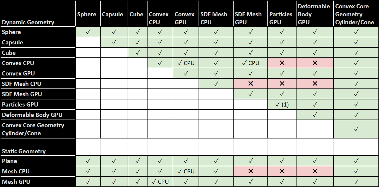
Figure 5 Rigid Body Collider Compatibility Table#
Table Notes
✓ CPU: compatible, running on CPU. See also performance consideration notes below.
✓ (1): Particles can collide within the same particle system, but cannot collide with particles that are in another particle system.
Collider Geometry Notes
Sphere: includes Mesh Bounding Sphere, and Sphere Approximation
Cube: includes Mesh Bounding Cube
Convex CPU: Convex Hulls are cooked for both CPU and GPU compatibility in general and automatically use the appropriate data and compute device depending on the simulation running on CPU or GPU. A CPU-only convex is generated if the input mesh data (before scaling) is oblong, in which case a warning will be issued in the console:
[Warning] [omni.physx.cooking.plugin] ConvexMeshCookingTask: failed to cook GPU-compatible mesh, collision detection will fall back to CPU. Collisions with particles and deformables will not work with this mesh. Prim /World/ConeMesh CPU: Triangle meshes are cooked for both CPU and GPU compatibility in general and automatically use the appropriate data and compute device depending on the simulation running on CPU or GPU. A multi-material triangle mesh is a CPU-only mesh.
Performance Considerations with CPU Collision Geometry
In general, CPU collision geometry generates contacts on the CPU, while GPU collision geometry generates contacts on the GPU. Most geometry supports both CPU and GPU, for example, Spheres or Convex Hulls (see note above), and automatically uses the appropriate compute device based on the simulation running on the CPU or on the GPU.
GPU-only features such as Deformable Bodies or Particles can only be used when GPU simulation is enabled. However, this is not true for some of the CPU-only collision geometry with GPU simulation. For example, a CPU-only convex hull can collide with a dynamic SDF Mesh. This is achieved by running the contact generation on CPU, which may incur a performance penalty, particularly for large GPU simulations such as reinforcement learning environments. In the table above, CPU/GPU collision pairs that are supported but run on the CPU are marked accordingly (✓ CPU).
Rigid Body Instancing#
USD supports two types of instancing:
Both approaches work with rigid bodies, but each has their own restrictions.
Note
Articulation links may not be instanced using neither scenegraph instancing nor UsdGeom.PointInstancer.
Scenegraph Instancing#
Rigid body scenegraph instancing permits scene hierarchies of collision geometry to be instanced without modification. More specifically, this feature allows collision geometry to be referenced so that many rigid bodies may share the same collision archetype.
The following Python snippet demonstrates how to use scenegraph instancing for rigid bodies:
from pxr import Usd, UsdGeom, UsdPhysics, Gf
import omni.usd

# Create a stage
omni.usd.get_context().new_stage()
stage = omni.usd.get_context().get_stage()

# Define the root Xform (transformable object)
rootxform = UsdGeom.Xform.Define(stage, "/World")

# Create a rigid body with two collider spheres.
# The two collider spheres will be referenced by multiple rigid bodies.
# Note that this would usually be prepared in a different USD file.
rigidBodyPath = "/World/rigidBody"
spheresRootPath = rigidBodyPath + "/theSpheres"
spherePaths = [spheresRootPath + "/sphere0", spheresRootPath + "/sphere1"]
spherePositions = [Gf.Vec3f(0, 2, 0), Gf.Vec3f(0, -2, 0)]
sphereRadii = [1, 2]
rigidBodyXform = UsdGeom.Xform.Define(stage, rigidBodyPath)
rigidBodyPrim = rigidBodyXform.GetPrim()
UsdPhysics.RigidBodyAPI.Apply(rigidBodyPrim)
massAPI = UsdPhysics.MassAPI.Apply(rigidBodyPrim)
massAPI.CreateMassAttr(1.0)
for i in range(2):
    sphereGeom = UsdGeom.Sphere.Define(stage, spherePaths[i])
    sphereGeom.CreateRadiusAttr(sphereRadii[i])
    sphereGeom.AddTranslateOp().Set(spherePositions[i])
    UsdPhysics.CollisionAPI.Apply(sphereGeom.GetPrim())

# Make three dynamic rigid bodies that have collision provided by
# references to the two spheres.
rigidBodyPaths = [
    "/World/theRigidBodies/rigidBody0",
    "/World/theRigidBodies/rigidBody1",
    "/World/theRigidBodies/rigidBody2"
]
rigidBodyStartPositions = [Gf.Vec3f(5, 0, 0), Gf.Vec3f(10, 0, 0), Gf.Vec3f(15, 0, 0)]
rigidBodyMasses = [2, 3, 4]
for i in range(3):
    rigidBody = UsdGeom.Xform.Define(stage, rigidBodyPaths[i])
    rigidBody.AddTranslateOp().Set(rigidBodyStartPositions[i])
    rigidBodyPrim = rigidBody.GetPrim()
    UsdPhysics.RigidBodyAPI.Apply(rigidBodyPrim)
    massAPI = UsdPhysics.MassAPI.Apply(rigidBodyPrim)
    massAPI.CreateMassAttr(rigidBodyMasses[i])
    # Configure with a reference to the two sphere colliders
    rigidBodyPrim.GetReferences().AddInternalReference(spheresRootPath)
    rigidBodyPrim.SetInstanceable(True)
The Python snippet begins by creating a rigid body with two sphere colliders. This is explained in more detail in section Configure a Rigid Body with multiple Colliders. With the y-axis as the up vector, there is a small sphere (radius=1) that is positioned above a larger sphere (radius=2). The snippet then goes on to create three more rigid bodies that take a reference to the sphere colliders of the original rigid body. This mechanism allows collision geometry to be defined once and then reused multiple times. A key point here is that this mechanism only allows collision geometry to be referenced.
The path hierarchy plays a crucial role. The rigid bodies created with references to collision geometry do so by making a reference to the hierarchy under “/World/rigidBody/theSpheres”:
rigidBodyPrim.GetReferences().AddInternalReference(spheresRootPath)
Only collision geometry in the above snippet is created under “/World/rigidBody/theSpheres”. In this case, there is only /World/rigidBody/theSpheres/sphere0 and /World/rigidBody/theSpheres/sphere1. As a consequence, the group of three rigid bodies created using references to collision geometry make references only to the two collision spheres and nothing else.
Scenegraph instancing allows only collision geometry to be referenced: rigid body parameters may not be referenced with this technique. This is seen in the above snippet, which gives a mass of 1.0 mass unit to the original body but a mass of 2.0, 3.0 and 4.0 mass units to the three bodies created with references to the collider spheres.
The outcome of the above snippet is four dynamic rigid bodies all sharing the same sphere collider attributes. Having shared the sphere colliders, it is not possible to modify their attributes. This is true of all collision types. If modification is a requirement then it is recommended to create individual collider instances.
Point Instancing#
This section introduces instancing of the entire rigid body. This makes use of UsdGeom.PointInstancer, as demonstrated in the following Python snippet:
from pxr import Usd, UsdGeom, UsdPhysics, Gf
import omni.usd

# Create a stage
omni.usd.get_context().new_stage()
stage = omni.usd.get_context().get_stage()

# Define the root Xform (transformable object)
rootxform = UsdGeom.Xform.Define(stage, "/World")

# Create the point instancer
pointInstancerPath = "/World/pointinstancer"
pointInstancer = UsdGeom.PointInstancer.Define(stage, pointInstancerPath)

# Create a  prototype rigid body with 2 collider spheres under pointInstancerPath
prototypeRigidBodyPath = pointInstancerPath + "/rigidBodyPrototype"
prototypeRigidBody = UsdGeom.Xform.Define(stage, prototypeRigidBodyPath)
prototypeRigidBody.AddTranslateOp().Set(Gf.Vec3f(0.0))
prototypeRigidBody.AddOrientOp().Set(Gf.Quatf(1.0))
prototypeRigidBodyPrim = prototypeRigidBody.GetPrim()
UsdPhysics.RigidBodyAPI.Apply(prototypeRigidBodyPrim)
massAPI = UsdPhysics.MassAPI.Apply(prototypeRigidBodyPrim)
massAPI.CreateMassAttr(2.0)
# Create two sphere colliders as children of the prototype rigid body.
prototypeRigidBodySpherePaths = [
    pointInstancerPath + "/rigidBodyPrototype/sphere0",
    pointInstancerPath + "/rigidBodyPrototype/sphere1"
]
prototypeRigidBodySpherePositions = [Gf.Vec3f(0, 2, 0), Gf.Vec3f(0, -2, 0)]
prototypeRigidBodySphereRadii = [1, 2]
for i in range(2):
    sphereGeom = UsdGeom.Sphere.Define(stage, prototypeRigidBodySpherePaths[i])
    sphereGeom.AddTranslateOp().Set(prototypeRigidBodySpherePositions[i])
    sphereGeom.CreateRadiusAttr(prototypeRigidBodySphereRadii[i])
    UsdPhysics.CollisionAPI.Apply(sphereGeom.GetPrim())

# Point instancer setup
# Add the prototype rigid body
prototypeList = pointInstancer.GetPrototypesRel()
prototypeList.AddTarget(prototypeRigidBodyPath)

# Setup the point instancer to create three instances of the prototype
prototypeIndices = [0, 0, 0]
rigidBodyStartPositions = [Gf.Vec3f(5, 0, 0), Gf.Vec3f(10, 0, 0), Gf.Vec3f(15, 0, 0)]
rigidBodyStartRotations = [Gf.Quath(1.0), Gf.Quath(1.0), Gf.Quath(1.0)]
rigidBodyStartLinVelocities = [
    Gf.Vec3f(0.0, 5.0, 0.0),
    Gf.Vec3f(0.0, 10.0, 0.0),
    Gf.Vec3f(0.0, 15.0, 0.0)
]
rigidBodyStartAngVelocities = [
    Gf.Vec3f(0.0, 30.0, 0.0),
    Gf.Vec3f(0.0, 60.0, 0.0),
    Gf.Vec3f(0.0, 90.0, 0.0)
]

# Configure the three instances with initial positions and velocities.
pointInstancer.GetProtoIndicesAttr().Set(prototypeIndices)
pointInstancer.GetPositionsAttr().Set(rigidBodyStartPositions)
pointInstancer.GetOrientationsAttr().Set(rigidBodyStartRotations)
pointInstancer.GetVelocitiesAttr().Set(rigidBodyStartLinVelocities)
pointInstancer.GetAngularVelocitiesAttr().Set(rigidBodyStartAngVelocities)
The snippet creates a scene that is similar to the scene created in Scenegraph Instancing but with a few key differences. The snippet begins by creating a rigid body with a mass of 2.0 mass units and two collider spheres of differing radii. This original rigid body may be viewed as a prototype that will be copied multiple times. The snippet then creates three rigid bodies as copies of the original prototype. As a consequence, properties of the prototype such as mass and collision geometry will be shared by the copies of the prototype rather than given individual values.
The snippet creates only three rigid bodies, the prototype is not added to the physics scene. Scengraph and point instancing, therefore, create different outcomes. With scenegraph instancing, the original geometry is added to the physics scene, while the prototype created with point instancing is not added to the physics scene.
The pose and velocity of rigid bodies created using point instancing may not be modified by directly addressing the pose and velocity attributes of UsdGeom.Xformable and UsdPhysics.RigidBodyAPI. Instead, the poses and velocities of the rigid bodies are updated using arrays, as shown in the above snippet.
Note
Rigid bodies created using point instancing may not have associated joints. To use joints with point instanced rigid bodies, it is necessary to use PhysxSchema.PhysxPhysicsJointInstancer.