Articulation and Robot Simulation Stability Guide#
This guide provides recommended practices for tuning articulation and simulation parameters to achieve stability in robot simulations.
Reduce Simulation Timestep for Complex Systems and Closed Loops#
Complex mechanical systems often have higher natural frequencies and require smaller timesteps for stable outcomes. For example, closed articulation loops often requires higher simulation frequency than the default 60Hz to run well. Humanoid robots are often simulated at 100Hz and more.
Experiment with reducing the simulation timestep to determine if the instability is resolved at smaller timesteps.
If stability emerges at a smaller timestep, experiment with reducing the number of TGS/PGS position iterations. This will improve performance and often stability is preserved with fewer iterations at smaller timesteps.
Mimic Joint Compliance#
Competing hard constraints can be a challenge for the solver algorithm; unstable robot simulations often feature a competing set of hard constraints such as contacts, very stiff joint drives, and mimic joints. Manipulation scenarios are particularly prone to these issues. Adding compliance to mimic joints can provide just enough yield to avoid numerical issues in the solver.
Mimic joint compliance is characterized with a natural frequency attribute and a damping ratio attribute. A tuning guide for these parameters and further stability considerations are available in Tuning a Compliant Mimic Joint.
Maximum Joint Velocity#
The early stages of RL training are often associated with high joint accelerations and velocities that can lead to instability.
Make use of the maximum joint velocity to clamp joint velocities promoting simulation stability in early training stages. Often, a generous limit of 200-300 deg/second for revolute joints can result in fewer simulation instabilities.
Maximum Drive Force#
Stiff drives can often lead to very large drive forces. This can become a stability issue when drive is combined with other stiff constraints such as non-compliant mimic joints and contacts.
The fundamental issue with stiff drives is that large forces lead to large accelerations and high velocities.
For linear degrees of freedom it is best to avoid accelerations that are orders of magnitude greater than gravitational acceleration.
For angular degrees of freedom it is best to avoid accelerations that result in velocities that produce rotations approaching 360 deg/second in a single simulation step.
Make use of the maximum drive force. This clamps the drive force that is applied to the joint.
Avoid maximum drive forces that would generate very large accelerations if applied to the smallest body mass or inertia component of the associated body pair.
Use the maximum output torque or force that is listed in the robot actuator specification, as available.
Drive Stability#
Badly tuned drives can generate instabilities, particularly when large drive stiffness are combined with small body masses or other competing hard constraints in the systems like contacts or mimic joints.
PD-control joint drives can be modelled as spring-dampers characterized with stiffness and damping attributes. It is possible to tune them to reasonable, stability-promoting values considering their associated natural frequency and damping ratio.
For linear drives, we have the following rough approximations:
naturalFrequency = sqrt(stiffness / mass)
dampingRatio = damping / (2 * sqrt(stiffness * mass))
with mass taken as the lightest mass of the body pair coupled by the joint, possibly considering the attached articulation subtree in the lightest mass calculation.
For angular drives, we have the complementary approximations:
naturalFrequency = sqrt(stiffness / inertia)
dampingRatio = damping / (2 * sqrt(stiffness * inertia))
with inertia taken as the smallest relevant inertia component of the body pair, possibly considering the attached articulation subtree in the inertia estimate.
Similar to mimic joint compliance, a key metric to consider when tuning is the product of natural frequency and simulation timestep.
Avoid simulation timestep and drive natural frequency combinations whose product is much greater than 1. This is particularly true if the driven joint participates in a mimic joint or participates in a gripping action.
Consider reducing the effective timestep with the TGS solver by increasing the number of position iterations. Alternatively, the simulation timestep may be reduced. Both choices come with a performance penalty. For recovering some performance, see also Reduce Simulation Timestep for Complex Systems and Closed Loops.
Values of damping ratio beyond the critical damping threshold will provide a steady approach to the equilibrium state but might be unnecessarily sluggish.
Use the stiffness and damping parameters listed in the robot actuator specification, as available.
Acceleration Drives#
If there is no information available from robot hardware about stiffness and damping (i.e. proportional and derivative gains) of the robot’s joint drives, it may be challenging to tune the drives to reasonable values even when following the tuning and stability advice above, which still holds for acceleration drives.
A key benefit of acceleration drives is that they are more straightforward to tune because the physics engine compensates for joint inertia at each time step and you can tune natural frequency and damping ratio directly with the below formulas. The simpler tuning approach often results in more reasonable drive forces that improve stability (but even with acceleration drives stability issues can arise).
For both angular and linear drives, you can compute stiffness and damping from natural frequency and damping ratio:
stiffness = naturalFrequency * naturalFrequency
damping = 2 * dampingRatio * sqrt(stiffness)
Note that since the simulation does not consider mass connected to a joint via contacts when computing the joint inertia per step, so acceleration drives may appear to be too weak in manipulation scenarios.
Joint Position Tracking Performance#
When using a drive to track a target position or velocity trajectory, one can be tempted to set very high stiffness gains to get close and quasi-kinematic target tracking. As mentioned above, this can lead to very large forces and lead to instability in more complex systems with competing hard or loop constraints, see above discussions on drive gains.
Improve tracking performance with reasonable stiffness values by adding feed-forward control effort such as gravity compensation, acceleration compensation, coriolis compensation. See the inverse dynamics helpers in the Tensor API documentation, e.g.
get_gravity_compensation_forces.Large forces can also be produced by setting position and velocity drive targets far from the current joint state. Consider setting an appropriate drive force limit, or implementing something like a rate-limiter on the drive targets.
Mass Ratios#
An impulse applied to a large mass can produce very large velocities when propagated to a body with small mass.
Avoid large mass and inertia ratios.
Use OmniPVD - PhysX Visual Debugger to inspect the masses and inertias of the articulation links and ensure that mass properties are setup to reasonable values, and nonzero in particular.
Joint Armature#
Joint armature can help with stability by adding joint-space inertia and corresponding damping.
If a geared actuator is modeled, you can set armature to represent reflected inertia of the motor rotor; armature should be set to JG2 with G denoting the ratio of motor angular velocity divided by the output shaft angular velocity, and J denoting the rotor inertia.
Articulation Link Self-Collision#
Unintended self-collisions between non-adjacent articulation links can be a source of instability.
When articulation self collision is enabled with physxArticulation:enabledSelfCollisions in PhysxSchema.PhysxArticulationAPI, PhysX automatically filters collisions between parent and child links. In the three-link articulation example below, PhysX automatically filters collisions between links A and B, and B and C. Note that these collisions are always filtered and cannot be enabled. However, non-adjacent links can still collide as shown in this example:
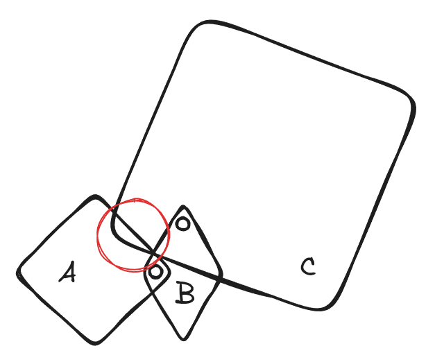
The collision geometry of links A and C is such that they collide, see red circle, which can lead to instability as the contact forces can cause high joint velocities.
Typically, self-collisions are important for modeling, so disabling self-collisions globally in PhysxSchema.PhysxArticulationAPI is not an option.
Instead, you can selectively disable self-collisions between the articulation links A and C, e.g. using UsdPhysics.FilteredPairsAPI, see Pairwise Collision Filtering.
This source of instability can be difficult to diagnose; a first step is to disable self-collisions to check if that resolves any observed instabilities. Then, you may use collision geometry visualization using Viewport Overlays and contact debug visualization using Physics Debug Window to diagnose self-collision issues.
Articulation Solver Order#
The solver has a strict ordering, as discussed here. For some gripping scenarios this might not be the best choice because the solver favors the contraint types that are resolved last. This is particularly true of stiff constraint systems that are hard to resolve without resorting to vanishingly small simulation timesteps.
With dynamic contact resolution being such an important part of gripping, it might make more sense to solve dynamic contact towards the end of the solver rather than at the beginning. This is achieved by raising a scene flag as follows:
from pxr import Usd,UsdPhysics,Sdf,PhysxSchema

stage = omni.usd.get_context().get_stage()

scene = UsdPhysics.Scene.Define(stage, "/physicsScene")
scenePrim = scene.GetPrim()
scenePrim.CreateSolveArticulationContactLastAttr().Set(True)
The snippet above reorders the solver so that
maximum joint velocity is enforced last.
dynamic contact is resolved immediately before static contact.
Moving dynamic contact towards the end of the solver sequence can lead to a reduction in persistent contact depth. Moreover, enforcing the maximum joint velocity at the very end of the sequence can lead to the contact constraints working harder to resolve joint velocities that are driven temporarily beyond the velocity limit. This can lead to stronger contact normal forces and stronger friction forces that aid gripping strength.
Raising the flag described here is an option to try if there is persistent contact penetration. Raising the flag does result in a measurable performance penalty. It may, however, lead to the desired outcome without resorting to the considerable expense of a reduced timestep.