Simulation Data Visualizer Window

Understanding how data changes overtime is important to fully analyze data and identify issues. By enabling the Omni PhysX UI extension, you get access to the Simulation Data Visualizer window, which allows you to visualize the data by plotting graphs of a physics object’s properties during simulation.

The feature is toggled through the viewport eye menu, for example:

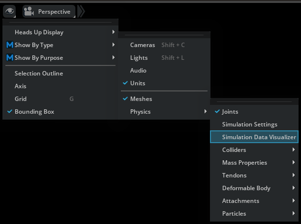
When enabled, a Simulation Data Visualizer window will appear docked in the bottom window group section.

By default, the window targets the currently selected prim or, if multiple prims are selected, the prim most recently added to the selection. However, it is possible to lock the window to a given prim by pressing the lock button:

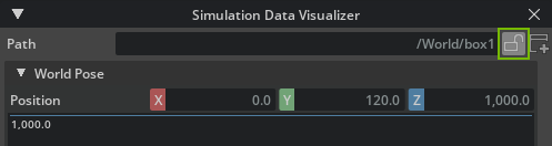
When the window is locked, it will keep targeting the same prim even as the current selection changes.

You can also create new Simulation Data Visualizer windows by pressing the new button:

Combined with the ability to lock windows, this enables you to monitor several prims at the same time by having multiple Simulation Data Visualizer windows open.

Note

When creating a new window, it will automatically set the old window to the locked state.

The contents of the individual windows will change based on what prim they are targeting. For example, a rigid body, joint, or residuals.

Rigid Bodies

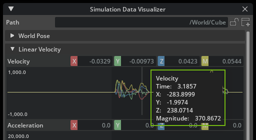
If the target is a rigid body, the window will show the following information:

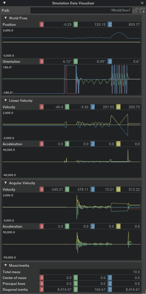
In the Velocity section, the M field (yellow) shows the magnitude of the velocity vector. That is, the current speed.

Also notice that the window provides some other simulation information that may not be observable through the regular property windows, for example current world pose and accelerations.

Note

Accelerations are derived from comparing the velocity between two discrete data samples, which yields the mean acceleration of the time delta rather than the current. However, given the high sample rate, the difference is usually negligible.

You can also inspect the mass and inertia properties of the rigid body, which is particularly useful if you have not set them explicitly and want to know the generated values (given that these are static throughout the simulation, they are not accompanied by graphs.)

Joints

When the window is targeting a joint prim, it will provide information about the current offsets, velocities, and accelerations in the local frame of the joint, that is, the values of the second attachment relative to the first:

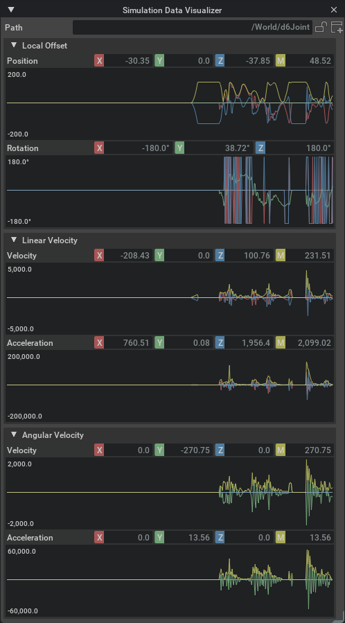
The exact values shown will change depending on the type of joint targeted.

Note

For joints, both velocities and accelerations are derived from comparing two discrete data samples, which yields the mean velocity and acceleration of the time delta. See the note above.

Residuals

The window will also visualize solver residuals if the targeted prim has the Residuals API applied:

These values provide an error metric that indicates the solver convergence in the respective part of the simulation (either the entire scene, an articulation root, or a single joint). When the values are zero, the solver converges perfectly.

Note

For joints, the RMS and Max values are always identical and therefore do not appear as separate properties and graphs.

Inspecting and Exporting Graph Data

Whenever a type of sampled data contains multiple components (for example, XYZ coordinates), you can toggle each of the subcomponents by left-clicking their label button:

In addition, you may also right-click a component, which will enable display of that specific component and hide all the others.

After the visualizer has plotted data in a graph, you can inspect the values at a specific data point by pressing the left mouse button while hovering it.

Further, if you right click the graph, all the samples for that plot will be copied to the clipboard in comma separated values format (CSV) that allows you to paste it into other database programs.