3.2. Jupyter Notebook

3.2.1. Learning Objectives

The goal of this tutorial is to familiarize you with the process of setting up and interacting with a live stage through the use of a jupyter notebook. Before getting started, you should complete the required tutorials and specifically familiarize yourself with Converting the Example to a Standalone Application.

10-15 Minute Tutorial

3.2.2. Getting Started

1. To begin, launch the following notebook.

   ./jupyter_notebook.sh standalone_examples/notebooks/scene_generation.ipynb

2. This may take several minutes if this is the first time jupyter_notebook.sh has been called.

3. Once the notebook is open, launch Isaac-Sim and navigate to localhost/Users/{user} in the content browser. Run cell 1 in the notebook and open temp_jupyter_stage.usd when it completes.

4. Once the stage is open (the context menu should be empty), activate live syncing by selecting Layer in the context pane and clicking the cloud icon. It should now say “Live Sync: ON” in the upper right corner of the editor window.

3.2.3. Interactive Development

Execute the next three cells and observe the stage as it updates in real-time as you call each cell. The last cell should generate and image like the following.

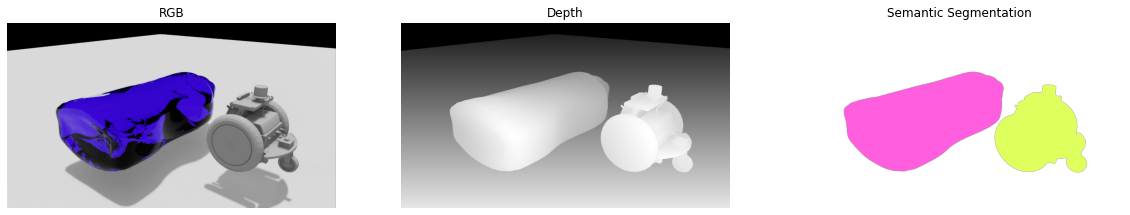
The stage can be modified by directly calling python commands in the notebook, and those changes will be executed live when the cell executes. Insert a cell before the one commented “cleanup application” and add the following to it.

carter_prim = stage.GetPrimAtPath(stage_path)
print(carter_prim)
xform_prim = XFormPrim(stage_path)
xform_prim.set_world_pose(position = np.array([0,1.0,0]))
simulation_world.render()

Execute the cell and the robot mesh will jump to y = 1.0 within the editor viewport, which is updated with the simulation_world.render() call. In this way, it’s possible to set up and verify a stage and its contents interactively through python. This process works in the other direction as well. In the context window for the interactive Omniverse Isaac Sim window, right-click and select Create > Mesh > Cone to create a cone at the origin. By default, the cone is created at /Cone, but note the path and insert another cell after the previous one.

cone_prim = stage.GetPrimAtPath('/Cone')
print(cone_prim)

Executing this cell returns Invalid null prim. Why? The file temp_jupyter_stage.usd is located on the nucleus server, which facilitates live synching. When simulation_app.step() is called, the simulation app updates itself with the changes from the stage. In the editor, this update call happens at a rate of about 120 Hz, but because we have manual control of the kit app, we are responsible for that. Adding a call to render() or step() will force this update to occur.

simulation_world.step()
cone_prim = stage.GetPrimAtPath('/Cone')
print(cone_prim)

This should now correctly return Usd.Prim(</Cone>)

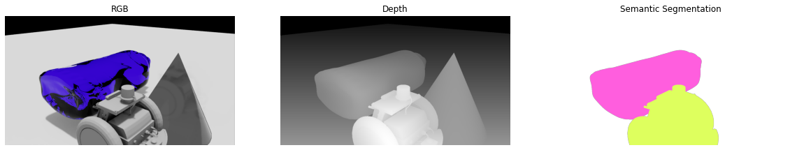
Finally, run the ground truth visualization cell (the fourth cell) to get new synthetic data from the updated scene.

3.2.4. Summary

This tutorial covered the following topics:

1. Updating the stage from a jupyter notebook

2. Working interactively with a scene through a jupyter notebook with live sync