11.1. Isaac Cortex: Overview

Cortex ties the robotics tooling of Isaac Sim together into a cohesive collaborative robotic system. Note that we are currently in a preview release and the APIs are experimental. Collaborative robotic systems are complex and it will take some iteration for us to get this right. We provide these tools to demonstrate where we’re headed and to give a sneak peak at the behavior programming model we’re developing.

11.1.1. Tutorial sequence

The Cortex tutorials start with an overview of the core concepts (this tutorial), and then step through a series of examples of increasing sophistication.

It’s best to step through the tutorials in order.

For more information, see Nathan Ratliff’s Isaac Cortex GTC22 talk

11.1.2. Overview of Cortex

Industrial robots do productive work by leveraging the robot’s speed and repeatability. Integrators structure the world around the robots so highly scripted behavior becomes a useful part of the workcell and assembly line. But these robots are often programmed only to move through their joint motions, and are generally unaware of their surroundings. That makes them easy to script, but also extremely unsafe to be around. These fast moving, dangerous, machines usually live in cages for safety to separate them from human workers.

Collaborative robotic systems are fundamentally different. These robots are designed to work in close proximity with people, uncaged, on the long tail of problems that require more intelligence and dexterity than can be addressed currently by scripted industrial robots. They need to be inherently reactive and adapt quickly to their surroundings (especially when human co-workers are nearby). But at the same time, we need them to remain easily programmable since their value is in the diversity of applications they can support. Cortex is a framework built atop Isaac Sim designed to address these issues. Cortex aims to make developing intelligent collaborative robotic systems as easy as game development.

Collaborative robotic systems typically have perception modules streaming information into a world model, and the robot must decide which skills to execute at any given moment to progress toward accomplishing its task. Often there are many skills to choose from. The robot must decide when to pick up an object, when to open a door, when to press a button, and ultimately which skills or sequence of skills are most suited to accomplish these steps. We’re, therefore, faced with the problem of organizing the available policies and controllers into an easily accessible API, and enabling straightforward programming of these decisions. Additionally, we want to do this in a way that enables users to develop first in simulation, then straightforwardly connect to perception and real-robot controllers for controlling physical robots.

The Cortex pipeline (detailed in the next section) revolves around leveraging the simulator as the world model. Isaac Sim has an expressive world representation based on USD with PhysX built on it, so this world model is both a detailed database of state information and physically realistic.

To easily switch between simulation and reality, we need to be able to modularly remove the perception component and operate directly on simulated ground truth during development. We also need to easily switch between controlling just the simulated robot and streaming commands to an external robot. Moreover, the decision framework should support reactivity as a first class citizen. All of these requirements are innately supported by Cortex as described below.

Advanced note

Modern deep learning techniques often learn abstract latent spaces encoding world information, but that doesn’t remove the need for a central database of information. We’re still a ways away from end-to-end trained systems that are robust and transparent enough to be deployed in production as holistic solutions. Until then, real-world systems will have many parts including perception modules and many policies representing skills that we need to orchestrate into a complete system. Even if each of these individual parts benefit from abstract latent spaces and its own perceptual streams (e.g. specialized skills with feedback), they still must be organized into a programmable coordinated system. Cortex is where the parts come together into a complete system.

11.1.2.1. The Cortex pipeline

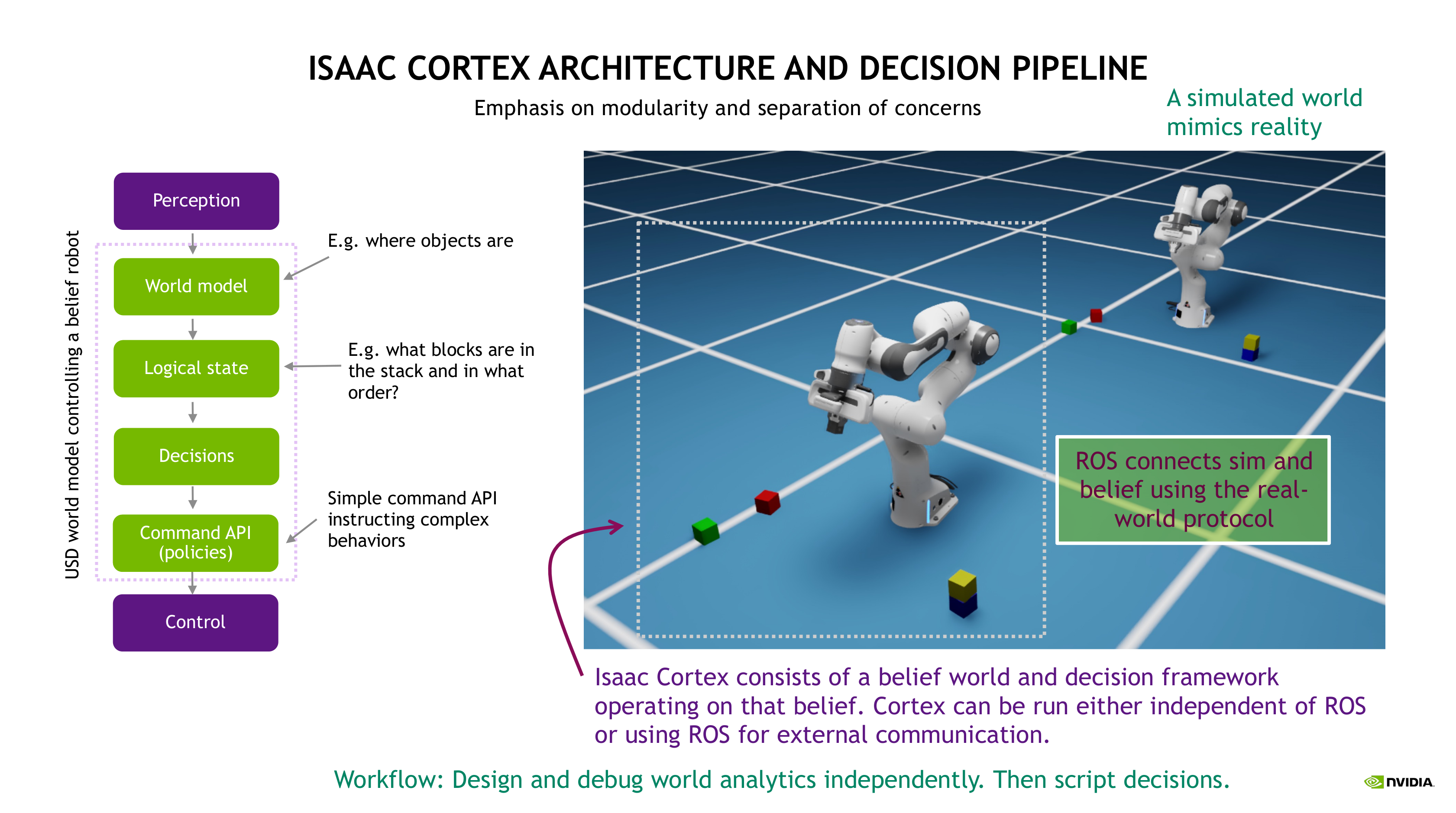
Cortex centers around a 6 stage processing pipeline which is stepped every cycle at 60hz (see also the diagram in the figure above):

Perception: Sensory streams enter the perception module and are processed into information about both what is in the world and where those objects are.
World modeling: This information is written into our USD database. USD represents our world belief capturing all available information. Importantly, this world model is visualizable, giving a window into the robot’s mind.
Logical state monitoring: A collection of logical state monitors monitor the world and record the current logical state of the environment. Logical state includes discrete information such as whether a door is open or closed or whether a particular object is currently in the gripper.
Decision making: Based on the world model and logical state, the system needs to decide what to do. What to do is defined by what commands are available through the exposed command API (see next item and below). The simplest form of decision model is a state machine. We build state machines into a new form of hierarchical decision data structure called a Decider Network which is based on years of research into collaborative robotics system programming at NVIDIA.
Command API (policies): Behavior is driven by policies, and each policy is governed by a set of parameters. E.g. motion with collision avoidance, is governed by sophisticated motion generation algorithms, but parameterized by motion commands that specify the target end-effector pose and the direction along which the end-effector should approach. Developers can expose custom command API for available policies to be accessed by the decision layer.
Control: And finally, low-level control synchronizes the internal robotic state with the physical robot for real time execution.

Layers 2 through 5 (world, logical, decisions, commands) operate on the belief model (the simulation running in the mind of the robot) and can be used entirely in simulation atop the Isaac Sim core API without any notion of physical (or simulated) reality. They enable complex systems to be designed in simulation first, focusing first on shaping the system’s behavior, before connecting to a physical (or simulated) world. Then perception can be added connecting into the world model via ROS and control can be added again connecting to the physical robot via ROS. Both of these stages can (and arguably should) be tested in simulation using simulated perception and control. For that purpose, we can use entirely separate simulated models with synthetic sensor data feeding into a real perception and control modules which will be running in practice. That allows us to adjust the noise characteristics, delays, and other real-world artifacts to profile and debug the end-to-end system thoroughly entirely before trying it in the physical world.

This concept of separate belief and sim (or real) worlds is fundamental to Cortex. Cortex operates on a simulation known as the belief (the mind of the robot). There may be a separate “external” simulation running as well which simulates the real world. Or (equivalently, as far as the belief simulation is concerned), the belief could be operating alongside the real physical world. Often we depict these two worlds with one robot in front of the other (see the figure above): the robot in front is the belief and the robot in back is the reality simulation.

Much of these tutorials focuses on the belief world in isolation. But see ROS Synchronization (Linux Only) for details on connecting to a simulated reality.

There are two extensions associated with Cortex:

omni.isaac.cortex: This extension handles layers 2 through 5 and is enabled by default with Isaac Sim.
omni.isaac.cortex_sync: This extension handles layers 1 and 6 including the ROS communication. It’s not available by default, but we show in our examples how to enable it and use the tools in standalone python apps (see ROS Synchronization (Linux Only)).

Currently, the Cortex programming model works only with the standalone Python app workflow.

11.1.2.2. A simple example

As an example, imagine you would like to have a robot arm follow a magical floating ball. In the world there is the robot, the ball, and a camera. Here is how the 6 stages of processing map to this robotics problem and world for each cycle:

Perception: An image is captured from the camera streamed and processed into the ball’s world transform, streamed as a tf via ROS to Cortex.
World modeling: The world is modeled in USD. The measured ball’s transform is recorded and made available to logical state monitors and behaviors which choose when and how frequently to synchronize the internal world model.
Logical state monitoring: A monitor is used to determine if the robot is gripping the ball. If the robot is gripping the ball the has_ball state is set to True, otherwise it is set to False.
Decision making: The ball’s current location, the robot’s current state, and the has_ball state are used in state machine to determine what the robot should do, either move towards the ball or do nothing.
Command API: If the robot should move towards the ball, the move towards the ball command is sent.
Control: Based on the commands received from the command API, low-level control commands are sent to the real robot via ROS.

The following video shows an example of stages 2 through 5 of this pipeline discussed in more depth in ROS Synchronization (Linux Only). For examples of 1 and 6 in simulation see ROS Synchronization (Linux Only).

11.1.3. Command API

PhysX represents robots in generalized coordinates as what are called articulations. In Isaac Sim, we wrap those into an Articulation class which provides a nice API for commanding the joints of the articulation. Those joint commands correspond to low-level control commands. But often policies will govern subsets of those joints to provide skills. For instance, a Franka arm’s articulation has 9 degrees of freedom, 7 for the arm and one for each of the two fingers. However, arm control on the physical robot is separate from the gripper control, with the gripper commands being discrete (move to position at a given velocity, close until the fingers feel a force).

Cortex provides a Commander abstraction which operates on a subset of the articulation’s joints and exposes an interface to sending higher-level commands to a policy governing those joints. A robot in the Cortex model is an articulation which has an associated collection of commanders governing the joints. For instance, a CortexFranka robot has a MotionCommander encapsulating the RMPflow algorithm governing the arm joints and a FrankaGripper commander governing the hand joints. Commands can be sent to commanders either discretely or at every cycle, and they’re processed by the commander into low-level joint commands every cycle. E.g. for the Franka, we can send a motion command (target pose with approach direction) and the commander will incrementally move the joints until it reaches that target. That target can either be changed every cycle (adapting to moving objects) or set just once; in either case, the motion commander will incrementally move the joints to the latest command.

The commanders along with their commands constitute the command API exposed for a given robot. For instance, if robot is a CortexFranka object, the two above mentioned commanders are exposed as robot.arm (the MotionCommander) and robot.gripper (the FrankaGripper), so anyone holding the robot object has access to the command APIs exposed by those commander objects. For instance, we can call robot.arm.send(MotionCommand(target_pose)) or its convenience method robot.arm.send_end_effector(target_pose) to command the arm, and we can call methods such as robot.gripper.close() to command the gripper.

Information about the latest command and the latest articulation action (low-level joint command) is cached off in the commander and accessible by modules in the control layer for translating those commands to the physical robot.

See CortexFranka in omni.isaac.cortex/omni/isaac/cortex/robot.py as an example of how these tools come together.

11.1.4. A note on rotation matrix calculations

In many of the examples, especially the complete examples stepped through in Walkthrough: Franka Block Stacking and Walkthrough: UR10 Bin Stacking we perform calculations on the end-effector or block transforms to calculate targets. To understand those blocks of code, note that a rotation matrix can be interpreted as a frame in a particulate coordinate system. Specifically, each column of the rotation matrix is an axis of the frame.

This is convenient when the axes have semantic meaning, such as for the end-effector. The Franka’s end-effector frame is as shown in the following figure with the x-, y-, and z-axes depicted in red, green, and blue, respectively.

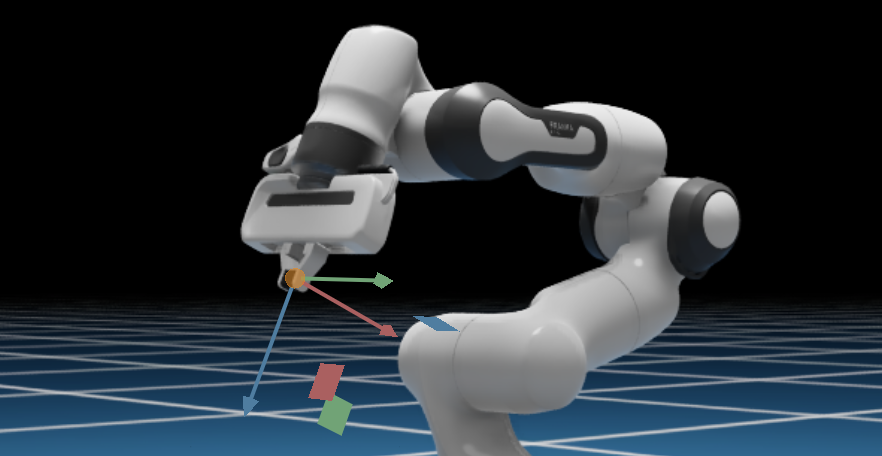
These x-, y-, and z-axes, as vectors in world coordinates, form the column vectors of the end-effector’s rotation matrix in world coordinates.

For instance, we might retrieve the end-effector’s rotation matrix and extract the corresponding axes using using:

import omni.isaac.cortex.math_util as math_util

R = robot.arm.get_fk_R()
ax,ay,az = math_util.unpack_R(R)

And we can compute the rotation matrix (target) that has the z-axis pointing down and maintains the most similar y-axis using:

import numpy as np

# Start with a z-axis pointing down. Project the end-effector's y-axis orthogonal to it (and
# normalize). Then construct the x-axis as the cross product.
target_az = np.array([0.0, 0.0, -1.0])
target_ay = math_util.normalized(math_util.proj_orth(ay, target_az))
target_ax = np.cross(target_ay, target_az)

# Pack the axes into the columns of a rotation matrix.
target_R = math_util.pack_R(target_ax, target_ay, target_az)

This type of math is common, and can be understood as simple geometric manipulations to an orthogonal frame.