Lidar Parameterization Tutorial: SICK TiM781#

This tutorial builds a working OmniLidar profile for the SICK TiM781-2174101 from public manufacturer documentation. It is a separate example from the Velodyne Alpha Prime tutorial: the Alpha Prime has many emitters per rotary tick, while the TiM781 has one measurement channel whose beam is swept by a rotating mirror.

The physical TiM781 is a rotating-mirror sensor, but the generic core can represent its scan in two useful ways:

SICK_TiM781.usda uses the ROTARY scheduler and models the mechanism with one emitter.
SICK_TiM781_SolidState.usda uses the SOLID_STATE scheduler and authors one nominal scan’s 811 explicit ray slots.

Both are source-based starting profiles, not certified digital twins of a particular hardware unit. The explicit profile assumes a full-period, scan-aligned capture; use the rotary profile when arbitrary render-step partitioning or rotation-boundary delivery matters.

Important

Treat the resulting USDA assets as deliberately vanilla, documentation-derived baselines. They contain what can be copied or reasonably inferred from the public manuals. Emitter and detector behavior that those sources do not define–including unit-specific optical power, receiver response and thresholds, noise, corrections, and intensity transfer–remains generic or approximate and must be tuned against measured sensor data for higher-fidelity use.

Source Documents#

This tutorial uses three SICK sources for order number TIM781-2174101 and part number 1096807:

TiM781-2174101 datasheet, accessed July 24, 2026. This is a dynamically generated German datasheet, despite sometimes being described as a manual.
TiM781 operating instructions, document 8024231/1ONO/2024-09-25.
TiM timestamp and index-signal explanation, SICK knowledge article KA-10209, version 1.0.

The short datasheet supplies the product envelope. The operating instructions add the measurement mechanism, telegram encoding, beam data, measurement origin, RSSI behavior, and timing needed to distinguish a physical encoder shot from an output sample. The knowledge article locates the TiM zero index and scan timestamp at -90 degrees.

Interpreting Source Confidence#

Each mapping below belongs to one of four categories:

Category	Meaning	How to use it
Direct	Source and simulation values have the same physical meaning and units.	Copy the value, then verify coordinate, boundary, and array conventions.
Derived	The source provides enough information to calculate the value.	Record the equation and source assumptions with the result.
Approximation	The source claim and generic-core model have different semantics.	Use it as an initial condition and validate against measurements.
Calibration	Public sources do not define the required value or transfer function.	Keep a documented starting value and replace it with measured data.

Read the Product-Level Specifications#

The operating instructions’ feature table provides the product envelope used by the profile.

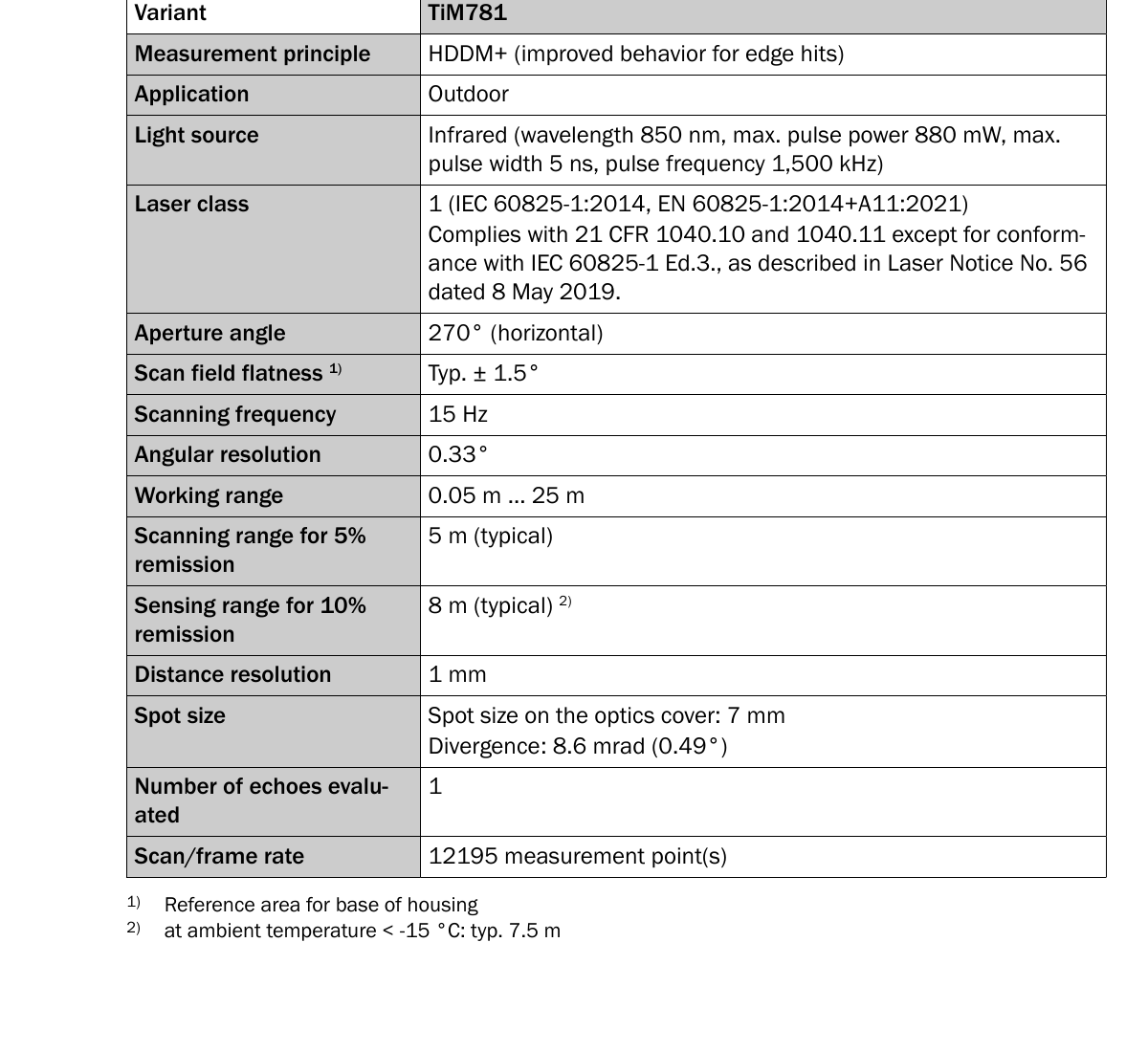
TiM781 feature table with scan, range, optical, and echo specifications — Excerpt from the TiM781 operating instructions, document 8024231/1ONO/2024-09-25, page 51.#

The complete source-to-model mapping is:

Manufacturer information	Simulation attribute or action	Value in this profile	Category	Notes
Rotating mirror with encoder-triggered angular increments	`scanType` and scheduling attributes	`ROTARY` mechanism or explicit `SOLID_STATE` frame	Approximation	`ROTARY` models the mechanism; `SOLID_STATE` can match its directions and per-ray offsets for a full-period, scan-aligned capture.
15 Hz scanning frequency	`tickRate`, `scanRateBaseHz`	`15`, `15`	Direct	One renderer period and one modeled scan period take about 66.667 ms.
Nominal 1/3-degree encoder step	`patternFiringRateHz` or solid-state azimuth array	Rotary: `16200`; solid state: `45 - i / 3`	Derived	The telegram encodes the repeating fraction as 0.3333 degrees; the explicit profile derives each angle directly.
Scan from -45 to +225 degrees	Rotary valid interval or explicit solid-state azimuth array	270-degree interval with 811 inclusive directions	Derived	Both preserve increasing SICK-angle order; the solid-state frame authors each direction explicitly.
One planar distance-data channel	`numberOfEmitters`, `numberOfChannels`	Rotary: `1`, `1`; solid state: `811`, `811`	Approximation	The TiM’s `DIST1` remains one physical channel; the solid-state profile assigns 811 analytic channel IDs to its explicit emitter slots.
0.05-25 m working range	`nearRangeM`, `farRangeM`	`0.05`, `25.0`	Direct	`rangeOffsetM` remains zero; it is not another name for minimum range.
1 mm distance resolution	`rangeResolutionM`	`0.001`	Direct	This is output granularity, not measurement accuracy.
Statistical error below 20 mm at 1 sigma	`rangeAccuracyM`	`0.02`	Approximation	The source condition is room temperature, at most 10 m, and 90% remission.
Systematic error of +/-60 mm	Validation target	Not authored as random error	Approximation	A signed, condition-dependent bias cannot be inferred from a symmetric bound.
Typical detection of 10% remission at 8 m	`minReflectance`, `minReflectionRangeM`	`0.10`, `8.0`	Approximation	The source says typical range, while the model pair describes a detection threshold. The 5%/5 m point remains a second validation target.
850 nm source	`waveLengthNm`	`850.0`	Direct	This affects spectral material response and photon conversion.
Up to 880 mW and up to 5 ns	`peakPowerW`, `pulseTimeNs`	`0.88`, `5`	Direct	They are not nominal calibrated operating values.
8.6 mrad single-pulse divergence and 5.8 mrad HDDM scan-width supplement	`divergenceHorDeg`, `divergenceVerDeg`	`0.8251`, `0.4927`	Approximation	The horizontal value represents the aggregate measurement footprint.
One evaluated echo	`maxReturns`	`1`	Direct	No multi-return capacity is needed.
Nonlinear, uncalibrated RSSI from 0 to 254	Intensity scale and calibration work	`254` with a linear starting map	Approximation	The public source does not provide the nonlinear transfer curve.
Measurement plane 62.46 mm above the housing-base reference	`emitterState:s001:vertOffsetM`	`0.06246` for each modeled emitter	Derived	The rotary array has one value and the solid-state array repeats it 811 times; the mounting asset must establish X/Y.

Build the Profile#

Start with an OmniLidar prim and apply the generic core API. The model metadata selects NVIDIA’s configurable model, while marketName identifies this product parameterization.

def OmniLidar "SICK_TiM781" (
    prepend apiSchemas = ["OmniSensorGenericLidarCoreAPI"]
)
{
    string omni:sensor:modelName = "LidarCore"
    string omni:sensor:modelVersion = "0.0.0"
    string omni:sensor:modelVendor = "NVIDIA"
    string omni:sensor:marketName = "SICK TiM781-2174101"
    float omni:sensor:tickRate = 15.0
    uint omni:sensor:Core:scanRateBaseHz = 15
}

tickRate controls the Kit sensor schedule, while scanRateBaseHz controls the generic core’s complete-scan period. Both the rotary and explicit solid-state assets set them to 15 Hz so the renderer schedule stays aligned with the TiM781 scan.

Choose the Generic-Core Scan Representation#

The operating instructions describe a rotating mirror and regular encoder-triggered measurements.

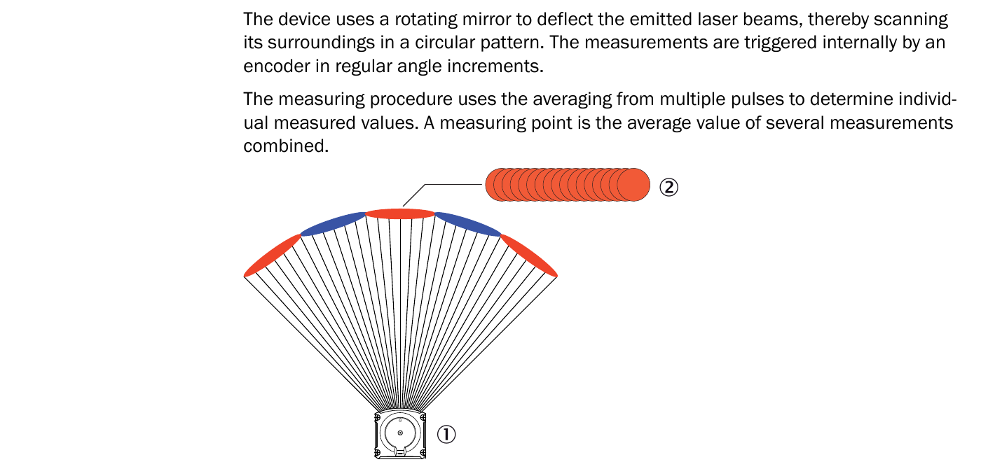
Excerpt from the TiM781 operating instructions, document 8024231/1ONO/2024-09-25, page 14. Each output measurement combines multiple pulses taken at an encoder-triggered angular increment.#

That physical fact does not require every simulation to use the rotary scheduler. Choose the representation according to which behavior the application needs:

Representation	Core structure	What it preserves	Prefer it when
Rotary mechanism	One emitter reused at 1080 candidate ticks per rotation; the visible field retains ticks 135 through 945	Persistent absolute rotary-scheduler phase across calls, zero-index alignment, scan-rate-derived cadence, and 811 visible samples	Mechanism fidelity, compact configuration, or changing scan rate matters
Explicit solid-state frame	811 virtual emitters in one line, each with an explicit direction and fire time	The same 811 directions and per-ray offsets at 15 Hz under a full-period, scan-aligned capture	A fixed ray layout is needed and final-emitter completion semantics are acceptable

SOLID_STATE is a generic-core scheduling abstraction in the second profile. It does not claim that the TiM781 hardware has a solid-state beam-steering mechanism.

Rotary Representation#

The rotary profile models the documented mechanism directly:

token omni:sensor:Core:scanType = "ROTARY"
token omni:sensor:Core:rotationDirection = "CCW"
uint omni:sensor:Core:patternFiringRateHz = 16200
uint omni:sensor:Core:numberOfEmitters = 1
uint omni:sensor:Core:numberOfChannels = 1

rotationDirection describes the simulated beam sweep after coordinate conversion. It is not a claim about the mechanical mirror-shaft direction, which the source does not name.

rotationDirection applies only to the rotary representation. For this profile, patternFiringRateHz / scanRateBaseHz gives 1080 ticks per rotation, or one tick every one-third degree. Do not author the solid-state-only numLines, numRaysPerLine, or emitterState:*:bank attributes in the rotary profile. Attributes not marked as exclusive in OmniSensorGenericLidarCoreAPI or its emitter-state API are common to both scan types.

Solid-State Representation#

The alternative profile authors the observable sweep as one explicit frame:

token omni:sensor:Core:scanType = "SOLID_STATE"
uint omni:sensor:Core:patternFiringRateHz = 15
uint omni:sensor:Core:numberOfEmitters = 811
uint omni:sensor:Core:numberOfChannels = 811
uint omni:sensor:Core:numLines = 1
uint[] omni:sensor:Core:numRaysPerLine = [811]

# Arrays below contain 811 values each.
float[] omni:sensor:Core:emitterState:s001:azimuthDeg = [...]
float[] omni:sensor:Core:emitterState:s001:elevationDeg = [...]
uint[] omni:sensor:Core:emitterState:s001:fireTimeNs = [...]
uint[] omni:sensor:Core:emitterState:s001:channelId = [...]
uint[] omni:sensor:Core:emitterState:s001:bank = [...]

The current solid-state implementation sizes output storage from numberOfChannels but indexes those slots by EmitterId. It therefore requires capacity for 811 channels even though the TiM has one physical distance-data channel. The explicit profile authors channelId from 1 through 811, producing output ChannelId values 0 through 810. This one-to-one analytic labeling matches EmitterId but does not imply 811 physical detector channels.

The solid-state schedule applies one explicit firing pattern per scan, so patternFiringRateHz equals scanRateBaseHz. rotationDirection is rotary-only. startAzimuthOffsetDeg and the valid-azimuth attributes are common, but the solid-state profile intentionally leaves them unauthored. The directions and scan window are already encoded in the emitter arrays.

Derive the Shared Scan Timing#

The operating instructions give 15 Hz, a nominal 1/3-degree step, and a 16.2 kHz measurement cadence:

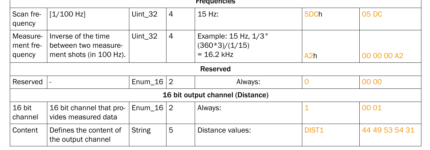
Excerpt from the TiM781 operating instructions, document 8024231/1ONO/2024-09-25, page 79. The telegram derives 16.2 kHz from 15 Hz and 1/3-degree increments and identifies one distance-data channel, DIST1.#

full_rotation_ticks = 360 / (1 / 3) = 1080
rotation_period = 1 / 15 = 66.6667 ms
tick_period = 1 / 16200 = 61.7284 us
visible_sweep_time = 810 * tick_period = 50 ms
blind_sector_time = 66.6667 ms - 50 ms = 16.6667 ms

There are 810 intervals and 811 inclusive angular bins from -45 to +225 degrees.

The telegram represents the repeating 1/3-degree value in units of 1/10000 degree as 3333, or 0.3333 degrees. The rotary profile uses the nominal encoder interpretation, approximately 360 / 1080, so the core snaps the schedule to 1080 ticks per rotation rather than treating the telegram’s quantized decimal as a phase-slipping physical step.

The explicit solid-state profile derives each direction and timestamp from the same nominal encoder sequence. For i = 0 .. 810:

sick_angle[i] = -45 + i / 3 degrees
authored_core_azimuth[i] = 45 - i / 3 degrees
fireTimeNs[i] = round((135 + i) * 1e9 / 16200)

Use absolute rounding as shown, rather than repeatedly adding a rounded tick period. The first and last fire times are 8,333,333 ns and 58,333,333 ns, with adjacent intervals alternating between 61,728 ns and 61,729 ns. The approximately 16.667 ms gap from the last visible point to the next frame’s first visible point represents the 90-degree blind sector.

The explicit pattern is tied to 15 Hz. If the simulated scan rate changes, regenerate its fire-time array; the rotary scheduler derives its cadence from the scan rate automatically.

Configure the Rotary Frame and Visible Sector#

SICK telegram samples run from -45 toward +225 degrees in positive increments. The scan timestamp is captured earlier, at the mirror’s -90-degree zero index. The generic core converts its authored azimuth to the right-handed Cartesian ray direction.

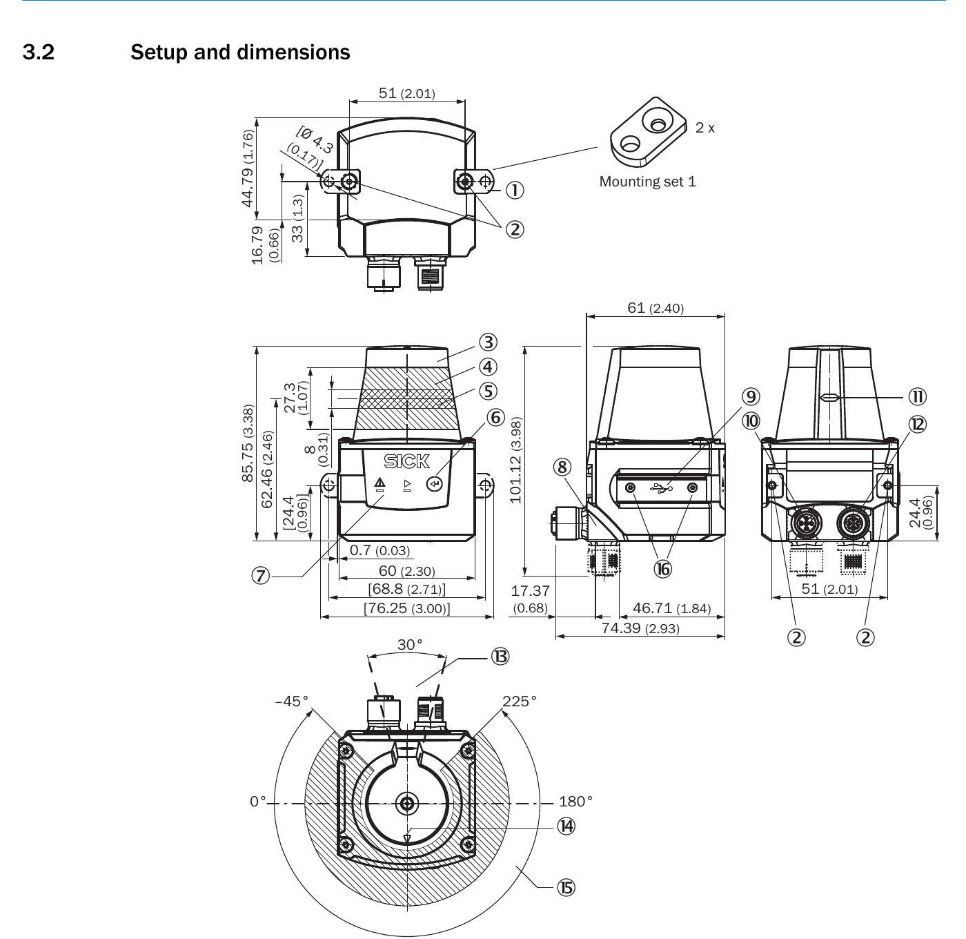
Figure 1 from the TiM781 operating instructions, document 8024231/1ONO/2024-09-25, page 11. The front view locates the scan plane 62.46 mm above the housing-base reference, and the plan view shows the -45 through +225-degree scan sector.#

The rotary profile uses:

token omni:sensor:Core:rotationDirection = "CCW"
float omni:sensor:Core:startAzimuthOffsetDeg = 90.0
float omni:sensor:Core:validStartAzimuthDeg = 44.9999
float omni:sensor:Core:validEndAzimuthDeg = 315.0001

At tick 0, the offset maps to the SICK -90-degree zero index and no visible ray is produced. Tick 135, about 8.333 ms later, is the first visible ray at -45 degrees. Tick 945, about 58.333 ms after the timestamp, is the last visible ray at approximately +225 degrees. The nominal internal valid interval is 45 through 315 degrees; the excluded sector splits the 16.667 ms blind time around the visible output.

These are nominal offsets. SICK specifies a +/-300 us tolerance for the timestamp taken at the zero index. Generic-core firing timestamps can additionally be displaced by less than one rotary tick, about 61.728 us here, because firing timestamps remain relative to the render-frame start rather than carrying an exact fractional absolute tick phase.

The profile expands both numerical endpoints by 0.0001 degree because valid boundaries are inclusive while the current clipped rotary capacity is calculated from ceil(sector_width / angular_step). The tiny epsilons retain both boundary ticks across float evaluation and reserve capacity for the 811th point without admitting another one-third-degree tick. Remove this accommodation when the clipped-capacity calculation accounts for both inclusive endpoints.

Define the Emitter Arrays#

The rotary profile applies one emitter pattern at every tick:

float[] omni:sensor:Core:emitterState:s001:azimuthDeg = [0.0]
float[] omni:sensor:Core:emitterState:s001:elevationDeg = [0.0]
float[] omni:sensor:Core:emitterState:s001:vertOffsetM = [0.06246]
uint[] omni:sensor:Core:emitterState:s001:fireTimeNs = [0]
uint[] omni:sensor:Core:emitterState:s001:channelId = [1]
uint[] omni:sensor:Core:emitterState:s001:rangeId = [0]

The SICK telegram’s DIST1 is one distance-data channel; the measurements within it are angular samples, not separate detector channels. Generic-core input channelId is one-based, so authored channel 1 produces PointCloud ChannelId 0.

The explicit solid-state profile stores all 811 ray slots in one emitter state:

# i = 0 .. 810; the downloadable asset expands every array.
azimuthDeg[i] = 45 - i / 3
elevationDeg[i] = 0
vertOffsetM[i] = 0.06246
fireTimeNs[i] = round((135 + i) * 1e9 / 16200)
channelId[i] = i + 1
rangeId[i] = 0
bank[i] = 0

The resulting PointCloud ChannelId and EmitterId both range from 0 through 810. This is a synthetic sample-slot identity; the physical telegram still contains one distance-data channel, DIST1.

The vertical offset assumes the prim origin is on the housing-base reference plane and maps only the Z separation to the optical plane. It is authored once in the rotary profile and repeated for all 811 explicit emitters in the solid-state profile. The source dimension does not by itself establish the prim’s lateral origin; the housing or mounting asset must define X/Y. If a mounting asset already places the prim at the marked optical origin, remove the emitter offset rather than applying the translation twice.

Configure Range and Error#

float omni:sensor:Core:nearRangeM = 0.05
float omni:sensor:Core:farRangeM = 25.0
float omni:sensor:Core:rangeResolutionM = 0.001
float omni:sensor:Core:rangeAccuracyM = 0.02
float omni:sensor:Core:minReflectance = 0.10
float omni:sensor:Core:minReflectionRangeM = 8.0
uint omni:sensor:Core:maxReturns = 1
uint omni:sensor:Core:rangeCount = 1
float[] omni:sensor:Core:rangesMinM = [0.05]
float[] omni:sensor:Core:rangesMaxM = [25.0]

rangeOffsetM is intentionally not set to 0.05 m. It makes nearby geometry invisible to avoid self-occlusion; nearRangeM is the attribute that represents the published minimum working range.

The 1 mm value is the reported distance increment. It does not force internal floating-point PointCloud coordinates to be quantized. The 20 mm value is a conservative approximation for the published statistical error, not a representation of the separate +/-60 mm systematic bound. Fit systematic bias with measured residuals rather than turning it into zero-mean random noise.

Configure Beam and Intensity Behavior#

token omni:sensor:Core:rayType = "IDEALIZED"
float omni:sensor:Core:waveLengthNm = 850.0
float omni:sensor:Core:divergenceHorDeg = 0.8251
float omni:sensor:Core:divergenceVerDeg = 0.4927
float omni:sensor:Core:peakPowerW = 0.88
uint omni:sensor:Core:pulseTimeNs = 5
token omni:sensor:Core:intensityProcessing = "NORMALIZATION"
token omni:sensor:Core:intensityMappingType = "LINEAR"
float omni:sensor:Core:intensityScalePercent = 254.0

The source gives 8.6 mrad single-pulse divergence and adds a 5.8 mrad scan-direction supplement when calculating the footprint of an HDDM measurement. The profile converts the aggregate 14.4 mrad horizontal and 8.6 mrad vertical footprints to degrees.

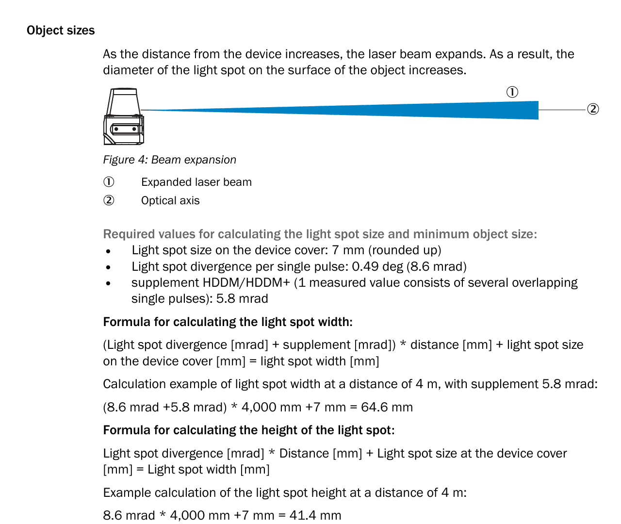
Figure 4 and its light-spot calculation from the TiM781 operating instructions, document 8024231/1ONO/2024-09-25, page 15.#

This is an approximation because the generic model does not average the sensor’s sequence of 1.5 MHz sub-pulses.

Divergence participates in radiometric calculations with the default IDEALIZED ray type. Start with that lower-cost representation. Use GAUSSIAN_BEAM only when geometric footprint and partial-hit fidelity are required and validated; it traces multiple rays and has a substantial performance cost.

The published 880 mW and 5 ns values are maxima. They are source-based starting points, but they remain calibration inputs rather than nominal unit measurements.

SICK RSSI is nonlinear, uncalibrated, and affected by remission, range, incidence angle, ambient light, temperature, and unit variation.

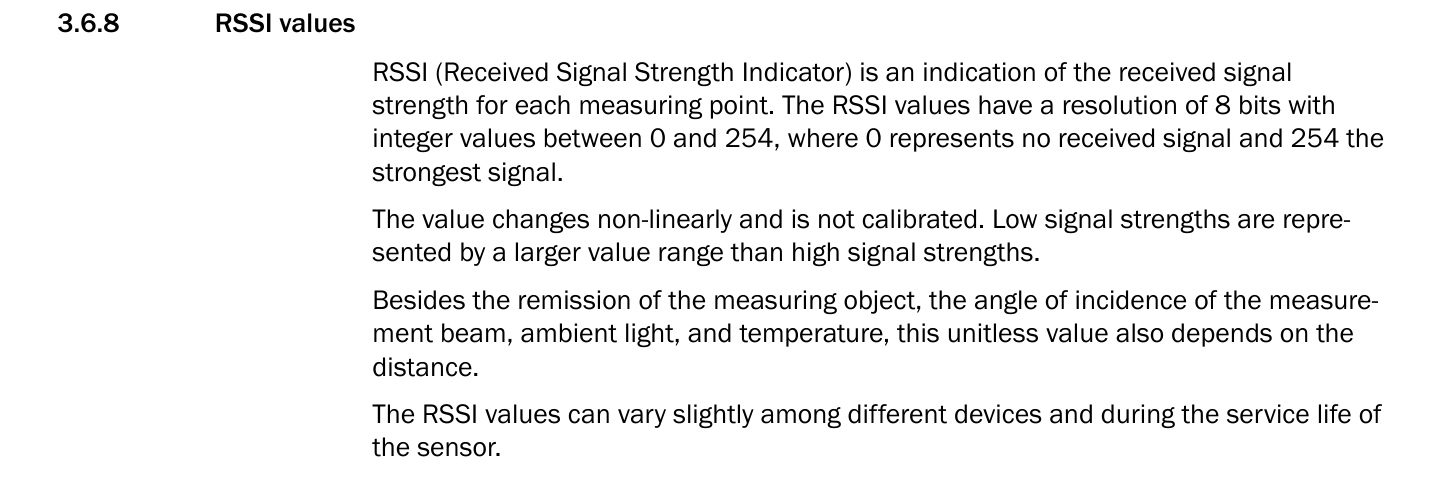
Excerpt from the TiM781 operating instructions, document 8024231/1ONO/2024-09-25, page 19.#

NORMALIZATION with a linear 0-254 starting map does not reproduce that transfer function. Fit a nonlinear encoding curve from paired sensor and simulation captures before claiming RSSI fidelity.

What Is Mappable and What Still Needs Work#

Easily Mappable or Uniquely Derivable#

The public documents support the following without unit-specific calibration:

15 Hz rate, nominal encoder cadence, visible sector, and blind-sector timing, represented either by rotary scheduling or an explicit frame;
one planar physical distance channel and one echo; the modeled emitter and channel counts depend on the selected scheduler;
minimum and maximum range, millimeter output resolution, wavelength, and the 10%/8 m detection anchor;
source-based optical maxima, nominal divergence, and the measurement-plane location;
RSSI range and the fact that the published RSSI mapping is nonlinear and uncalibrated.

Published but Not One-to-One#

Published behavior	Model or source limitation	Recommended treatment
12,195 measurement points per second	At 15 Hz this implies 813 points per scan, while -45 to +225 at nominal 1/3-degree increments gives 811 inclusive bins	Keep the documented geometry in this profile and verify the actual telegram count and outer angles on hardware.
Telegram step 0.3333 degrees	The telegram cannot exactly encode the stated repeating 1/3-degree encoder step	Use 1080 ticks per rotation; use a captured scan to determine whether firmware introduces any phase or boundary variation.
Statistical error below 20 mm and systematic error +/-60 mm	`rangeAccuracyM` controls distance-dependent Gaussian uncertainty	Use 0.02 m as a statistical starting scale and fit signed bias separately.
8.6 mrad pulse divergence plus HDDM scan-width supplement	One generic beam cannot reproduce multi-pulse averaging	Use the aggregate footprint as an approximation and validate small-object and edge-hit behavior.
5%/5 m and 10%/8 m detection points	The generic model has one threshold anchor	Use 10%/8 m as the profile anchor and retain 5%/5 m as an independent validation point.
Nonlinear 0-254 RSSI	No public transfer curve is supplied	Fit intensity mapping from calibrated remission targets across range and incidence angle.
Typical scan-field flatness of +/-1.5 degrees	Flatness is a systematic shape tolerance, not a random elevation distribution	Keep angular jitter at zero until a measured scan-plane correction or distribution is available.

Not Published and Requiring Calibration#

The documents do not uniquely define detector aperture and efficiency, intensity gain, the exact RSSI curve, per-unit angular and distance corrections, random angular-error distributions, temperature-dependent bias, or the nominal values behind the published optical maxima. Measure those terms on the target unit.

The real device can apply edge, particle, median, and averaging filters. These alter or suppress measurements and cannot be reconstructed from already filtered output. Match the device filter configuration before comparing captures with an unfiltered generic-core profile, or reproduce the selected filtering in post-processing.

Published but Outside the Generic Lidar Core#

Supply voltage, power consumption, enclosure protection, operating temperature, Ethernet and USB transport, field evaluation, digital I/O, and filter configuration are useful integration requirements but are not generic Lidar-core parameters. Represent physical housing geometry in mounting, visual, and collision assets, and represent transport or perception filtering in their corresponding systems.

Use the Asset#

Choose one of the two complete profiles:

SICK_TiM781.usda for the rotary mechanism representation.
SICK_TiM781_SolidState.usda for the explicit solid-state frame representation.

This example references the rotary profile’s default prim:

#usda 1.0
(
    defaultPrim = "World"
    metersPerUnit = 1
    upAxis = "Z"
)

def Xform "World"
{
    over "TiM781" (
        prepend references = @./SICK_TiM781.usda@
    )
    {
        double3 xformOp:translate = (0, 0, 0.5)
        uniform token[] xformOpOrder = ["xformOp:translate"]
    }
}

The untyped over preserves the referenced OmniLidar type. To use the explicit profile, change the reference filename to SICK_TiM781_SolidState.usda; its default prim is /SICK_TiM781_SolidState.

Both assets expose GenericModelOutput and PointCloud for convenience. Applications typically keep one output, remove the unused render variable, and request only the channels they consume.

accumulateOutputs = true matches the real sensor’s complete-scan telegram more closely by withholding output until a modeled scan is complete. Use partial output only when render-frame chunks are required by the application. For the explicit solid-state profile, use a full-period, scan-aligned capture or render-step partitions that include scheduled emitters. The current solid-state scheduler determines completion from the final emitter rather than the nominal frame end, and intervals wholly inside the authored blind gap are not a robust partitioning mode. Prefer the rotary profile when arbitrary render-step partitioning is needed.

For moving sensors or targets, enable renderer Motion BVH. The default NONCOMPENSATED output is raw scan data with motion effects, similar to a real sensor. COMPENSATED applies the motion-compensation step commonly performed near the beginning of perception stacks and is especially important for mapping.

Validate the Asset#

Checker Preflight#

Run the sensor checker in the Kit Sensors app, or another Kit app that enables omni.sensors.nv.common and exposes its bundled sensor_checker module:

import sensor_checker as sc
from pxr import Usd

model = sc.ModelInfo()
model.modelName = "lidar.core"
model.modelVersion = "1.0"
model.schemaVersion = "1.0"
model.modelVendor = "nv"
model.marketName = "SICK TiM781-2174101"

profiles = [
    ("/path/to/SICK_TiM781.usda", "/SICK_TiM781"),
    (
        "/path/to/SICK_TiM781_SolidState.usda",
        "/SICK_TiM781_SolidState",
    ),
]

for asset_path, prim_path in profiles:
    # Use a fresh checker because the two profiles have different
    # scheduler-specific parameter sets.
    checker = sc.SensorCheckerUtil()
    error = checker.init(model)
    if error:
        raise RuntimeError(f"Failed to initialize the Lidar checker: {error}")

    stage = Usd.Stage.Open(asset_path)
    prim = stage.GetPrimAtPath(prim_path)
    if not prim:
        raise ValueError(f"Missing Lidar prim {prim_path} in {asset_path}")

    error = checker.validateParams(prim)
    if error:
        raise ValueError(f"Invalid Lidar parameters in {asset_path}: {error}")

    schedule = checker.getSchedulerInfo()
    if schedule.errorString:
        raise ValueError(
            f"Invalid Lidar schedule in {asset_path}: "
            f"{schedule.errorString}"
        )

    if prim_path == "/SICK_TiM781_SolidState":
        prefix = "omni:sensor:Core:"
        emitters = prim.GetAttribute(
            prefix + "numberOfEmitters"
        ).Get()
        channels = prim.GetAttribute(
            prefix + "numberOfChannels"
        ).Get()
        channel_ids = prim.GetAttribute(
            prefix + "emitterState:s001:channelId"
        ).Get()
        assert emitters == channels == 811
        assert list(channel_ids) == list(range(1, channels + 1))

print("Both SICK TiM781 profiles are valid")

Geometry and Timing Checks#

Use a simple static scene first:

Check	Test setup	Expected result
Coordinate orientation	Place narrow targets at SICK angles -45, 0, 90, 180, and 225 degrees	For both profiles, the first visible sample is -45 degrees and samples proceed toward +225 degrees.
Scan rate	Run with a stable simulation clock for several seconds	15 complete scans per second; the rotary representation also completes 15 modeled rotations per second.
Encoder cadence	Inspect rotary candidate ticks or differences between solid-state `fireTimeNs` values	Rotary: 1080 ticks per rotation. Solid state: 811 explicit ray slots. Both use approximately 61.728 us between adjacent visible samples.
Visible timing	Inspect PointCloud `TimeOffsetNs` across a complete output	Both nominal schedules span approximately 8.333-58.333 ms relative to the assumed -90-degree scan timestamp. The source permits +/-300 us at the index; the rotary core can add less than one modeled tick of displacement.
Output completion	Compare scan-ready status with the nominal 66.667 ms period boundary	Rotary completion follows the rotation boundary. Solid-state completion follows inclusion of emitter 810; use a full-period, scan-aligned capture when equivalent delivery timing is required.
Point count	Count output angular bins in a surrounding wall scene	811 bins for either profile’s inclusive -45 to +225 interpretation; compare this with a real telegram because the published 12,195 points/s claim implies 813.
Channel identity	Request PointCloud `ChannelId`	Rotary: every point is channel 0. Solid state: channel IDs 0-810 correspond to the explicit ray slots.
Emitter identity	Request PointCloud `EmitterId`	Rotary: every point is emitter 0. Solid state: emitter IDs 0-810 correspond to the explicit ray slots.
Measurement origin	Place a surveyed wall and compare mounting-base and optical-plane transforms	Rays originate 62.46 mm above a prim placed at the assumed housing base.

Range and Intensity Checks#

Use surveyed, flat targets:

Verify rejection below 0.05 m and beyond 25 m.
Compare mean bias and residual spread at several ranges rather than treating +/-60 mm as a Gaussian sigma.
Check a 10% remission target at 8 m and retain 5% at 5 m as a second target.
Confirm one echo for partial occlusions and layered geometry.
Compare 0-254 RSSI distributions over remission, range, and incidence angle; replace the linear map only after collecting enough paired data.
Test narrow objects and depth edges with IDEALIZED first. Evaluate GAUSSIAN_BEAM only if aggregate-footprint behavior is important enough to justify its additional ray cost.

Compare with Real Sensor Data#

Capture raw, unfiltered LMDscandata from a stationary TiM781 with RSSI enabled. For each scan, record the reported start angle, angular step, sample count, device timestamp, distance, and RSSI. Use the capture to resolve the 811-versus-813 ambiguity and then compare:

angular order, boundary samples, scan cadence, and blind interval;
range bias and spread by distance and remission;
dropout probability and small-object/edge-hit behavior;
RSSI distributions;
temperature dependence and scan-plane shape.

Keep directly sourced geometry and timing fixed unless the capture shows that the published interpretation is wrong. Tune approximation and calibration parameters separately so a radiometric mismatch is not hidden by changing scan geometry.

Result and Limitations#

The completed assets provide two encodings of the same physical scan. The rotary profile models the mechanism compactly with one emitter and persistent absolute scheduler phase across calls. The solid-state profile provides an explicit 811-slot frame with the same nominal directions and per-ray offsets at 15 Hz for a full-period, scan-aligned capture. Both use the 10%/8 m detection anchor, published optical upper bounds, the documented measurement origin, and current user-facing outputs.

The remaining uncertainty is explicit. The published point-rate claim does not reconcile with the angular geometry; the exact RSSI transfer, HDDM multi-pulse processing, filter behavior, systematic range bias, scan-plane correction, and per-unit calibration require real sensor data. The explicit solid-state profile does not model rotary scheduler phase or rotation-boundary completion, and its fire-time array must be regenerated if its frame rate changes.