Lidar Parameterization Tutorial: Velodyne Alpha Prime#

This tutorial builds a working OmniLidar profile for the Velodyne Alpha Prime (VLS-128) from public sensor documentation. It shows how to distinguish values that map directly to the generic Lidar model, values that must be derived, published claims that only approximate a model parameter, and behavior that still requires calibration data.

The completed profile is available as Velodyne_Alpha_Prime_Rev4.usda. It is a source-based starting profile, not a certified digital twin of a particular hardware unit.

Important

Treat the resulting USDA as a deliberately vanilla, documentation-derived baseline. It contains what can be copied or reasonably inferred from the public manuals. Emitter and detector behavior that those sources do not define–including unit-specific optical power, receiver response and thresholds, noise, corrections, and intensity transfer–remains generic or approximate and must be tuned against measured sensor data for higher-fidelity use.

Source Documents#

This tutorial uses these exact manufacturer documents:

Alpha Prime Rev. 4 User Manual, document 63-9483 Rev. 2, last updated February 14, 2019. The title inside the PDF is VLS-128 User Manual.
Alpha Prime Datasheet, document 63-9679 Rev-B, published in 2021.

The manual’s Appendix A explicitly moves product specifications to the separate datasheet. The two files therefore form one source set: the manual defines packet layout, firing order, timing, coordinates, return behavior, and nominal channel angles; the datasheet supplies range, accuracy, field of view, frame-rate, detection, optical, electrical, and environmental specifications.

When the revisions differ, this tutorial uses the newer datasheet for product-level specifications and the manual for detailed VLS-128 operation. The one material conflict is wavelength: the manual describes 903 nm channels while the newer datasheet specifies approximately 905 nm. The profile uses 905 nm and records the difference so a profile for older hardware can use 903 nm instead.

The public ROS VLS-128 calibration file was examined only as an implementation cross-check. Its nominal angles match Figure 9-8 in the manual, and its additional distance, focal, and origin corrections are zero. It is not a manufacturer specification, does not provide per-unit factory calibration, and is not used as the source for this profile.

Interpreting Source Confidence#

Each mapping below belongs to one of four categories:

Category	Meaning	How to use it
Direct	The source value and simulation attribute have the same physical meaning and units.	Copy the value, then verify units, coordinate conventions, and array order.
Derived	The source contains enough information to calculate the simulation value uniquely.	Keep the equation and source assumptions next to the result.
Approximation	A published claim exists, but the simulator uses a different statistical or physical model.	Use the published value as an initial condition, then validate and tune against measurements.
Calibration	The public sources do not define the value, or a particular hardware unit can differ.	Start from a documented model default and replace it with measured or unit-specific data.

Read the Product-Level Specifications#

The datasheet’s sensor and laser table provides the high-level envelope used by the profile.

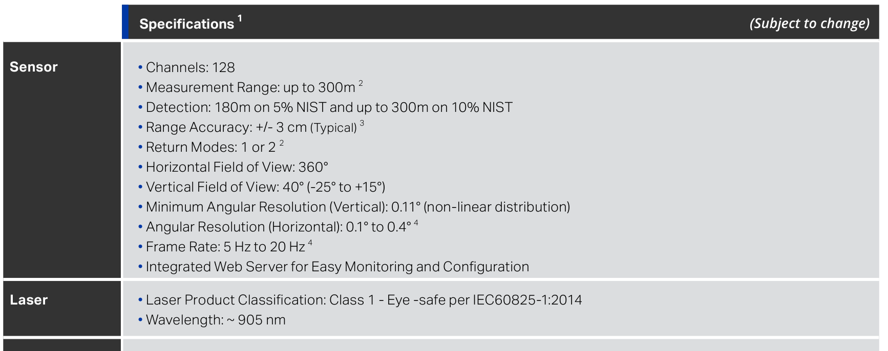
Alpha Prime Rev-B datasheet sensor and laser specification rows — Excerpt from the Alpha Prime datasheet, 63-9679 Rev-B, page 2.#

The complete source-to-model mapping is:

Manufacturer information	Simulation attribute or action	Value in this profile	Category	Notes
128 channels	`numberOfEmitters`, `numberOfChannels`	`128`, `128`	Direct	One nominal emitter maps to one detector channel.
Rotating VLS-128 architecture	`scanType`, `rotationDirection`	`ROTARY`, `CW`	Direct	The manual’s azimuth increases clockwise from its zero axis.
600 RPM selected from the 300-1200 RPM range	`tickRate`, `scanRateBaseHz`	`10`, `10`	Derived	Complete scans per second equal RPM divided by 60; the renderer and model rates are kept aligned.
53.3 us average firing sequence at 600 RPM	`patternFiringRateHz`	`18760`	Derived approximation	The reciprocal cadence is 18,761.726 Hz. The rotary core uses an integer number of ticks per scan, so this profile selects the nearest multiple of 10 Hz.
360-degree horizontal field of view	`validStartAzimuthDeg`, `validEndAzimuthDeg`	`0.0`, `360.0`	Direct	Runtime field-of-view clipping can narrow this interval.
40-degree vertical field of view, -25 to +15 degrees	`emitterState:s001:elevationDeg`	128-value non-linear array	Direct	Use Figure 9-8 rather than a uniformly spaced approximation.
Per-laser `AziOffset` values	`emitterState:s001:azimuthDeg`	Eight offsets repeated for 16 firing groups	Direct	Preserve the signs after aligning the coordinate frames.
Groups of eight every 2.665 us, with maintenance periods	`emitterState:s001:fireTimeNs`	128 derived offsets	Derived	Packet timestamp adjustment is not part of this array.
4 mm distance-field granularity	`rangeResolutionM`	`0.004`	Direct	This is packet/reporting resolution, not the accuracy distribution.
Measurement range up to 300 m	`farRangeM`	`300.0`	Direct	Datasheet footnote says configuration dependent.
Typical range accuracy of +/-3 cm	`rangeAccuracyM`	`0.03`	Approximation	The model uses a distance-dependent Gaussian error scale, not a guaranteed bound.
Detection at 180 m on a 5% NIST target	Validation target	5% at 180 m	Approximation	Retain this published point as a secondary validation check.
Detection up to 300 m on a 10% NIST target	`minReflectance`, `minReflectionRangeM`	`0.10`, `300.0`	Direct anchor	Use the farthest published detection point for the model’s single threshold anchor.
One or two returns	`maxReturns`	`2`	Direct	Strongest/last selection policy is separate from return capacity.
Dual returns recorded for surfaces at least 1 m apart	`minDistBetweenEchosM`	`1.0`	Direct	From the manual’s dual-return behavior.
Horizontal and vertical beam divergence	`divergenceHorDeg`, `divergenceVerDeg`	`0.1197482`, `0.06016057`	Direct	Values are published in both mrad and degrees.
Approximately 905 nm in the newer datasheet	`waveLengthNm`	`905.0`	Direct, revision-specific	Use 903 nm when targeting the older manual/hardware definition.
Calibrated reflectivity byte from 0 to 255	`intensityScalePercent`	`255.0`	Direct scale	The transfer curve still requires calibration.
Data origin 66.11 mm above the sensor base	`emitterState:s001:vertOffsetM`	128 values of `0.06611`	Direct	Places every emitter origin relative to a sensor prim located at the mechanical base.

Build the Profile#

Start with an OmniLidar prim and apply the generic core API. The model metadata selects NVIDIA’s configurable Lidar model; marketName identifies this parameterization, not a different simulation plugin.

def OmniLidar "Velodyne_Alpha_Prime_Rev4" (
    prepend apiSchemas = ["OmniSensorGenericLidarCoreAPI"]
)
{
    string omni:sensor:modelName = "LidarCore"
    string omni:sensor:modelVersion = "0.0.0"
    string omni:sensor:modelVendor = "NVIDIA"
    string omni:sensor:marketName = "Velodyne Alpha Prime Rev 4 (VLS-128)"
    float omni:sensor:tickRate = 10.0
    uint omni:sensor:Core:scanRateBaseHz = 10
    uint omni:sensor:Core:patternFiringRateHz = 18760
}

tickRate controls how often Kit schedules the sensor, while scanRateBaseHz controls the modeled complete-scan period. Keep them equal for this complete profile so one scheduled sensor period and one modeled rotation both represent the selected RPM.

Choose a Rotation Rate#

The manual permits 300 through 1200 RPM in increments of 60 RPM. For a rotary sensor:

scan_rate_hz = rpm / 60
exact_firing_rate_hz = 1 / 53.3e-6
ticks_per_scan = round(exact_firing_rate_hz / scan_rate_hz)
firing_rate_hz = ticks_per_scan * scan_rate_hz
angular_step_deg = 360 / ticks_per_scan

At 600 RPM, scan_rate_hz is 10. The reciprocal firing cadence is 18,761.726 Hz. The rotary core uses integer division to determine the number of ticks in a complete scan, so a fractional ratio does not add another tick to that scan. Select the closest firing rate that is divisible by the scan rate: patternFiringRateHz = 18760. This produces exactly 1876 ticks per scan and an angular advance of approximately 0.19189765 degrees per tick. The same derivation gives the manual’s operating points:

Motor speed	`scanRateBaseHz`	`patternFiringRateHz`	Derived angular step
300 RPM	5	18760	0.09594883 degrees
600 RPM	10	18760	0.19189765 degrees
900 RPM	15	18765	0.28776978 degrees
1200 RPM	20	18760	0.38379531 degrees

Recompute both rates when selecting another supported motor speed. The small variation in patternFiringRateHz keeps the modeled cadence close to the manual’s 53.3 us average while ensuring an integral number of ticks per scan.

At 10 Hz, the authored rates produce exactly 18760 / 10 = 1876 firing-pattern ticks per modeled rotation and 18760 * 128 = 2,401,280 candidate single-return measurements per second. This is 0.0092% below the exact reciprocal cadence of 18,761.726 Hz. The quantization is required to keep complete scans coherent with the generic Lidar core’s integer-rate scheduler. The datasheet’s approximately 2.3 million figure is a rounded product-output claim; valid output points can also be reduced by range, field-of-view, reflectance, and scene misses.

Align the Coordinate Frames#

Figure 9-1 in the manual defines zero azimuth along the sensor’s +Y axis and increases azimuth clockwise toward +X. The generic model’s unshifted zero direction is +X, so the profile uses:

token omni:sensor:Core:rotationDirection = "CW"
float omni:sensor:Core:startAzimuthOffsetDeg = 270.0

After this frame alignment, copy the manual’s AziOffset signs directly into emitterState:s001:azimuthDeg. For example, the manual’s laser ID 0 remains -6.354 degrees and laser ID 7 remains +6.354 degrees. Do not negate the table merely because Cartesian rendering uses a right-handed frame; the core model performs that conversion after applying the market-frame offset.

Map the Channel Pattern#

The 40-degree vertical field of view is not uniformly distributed. Figure 9-8 supplies the nominal azimuth offset and elevation for every laser ID.

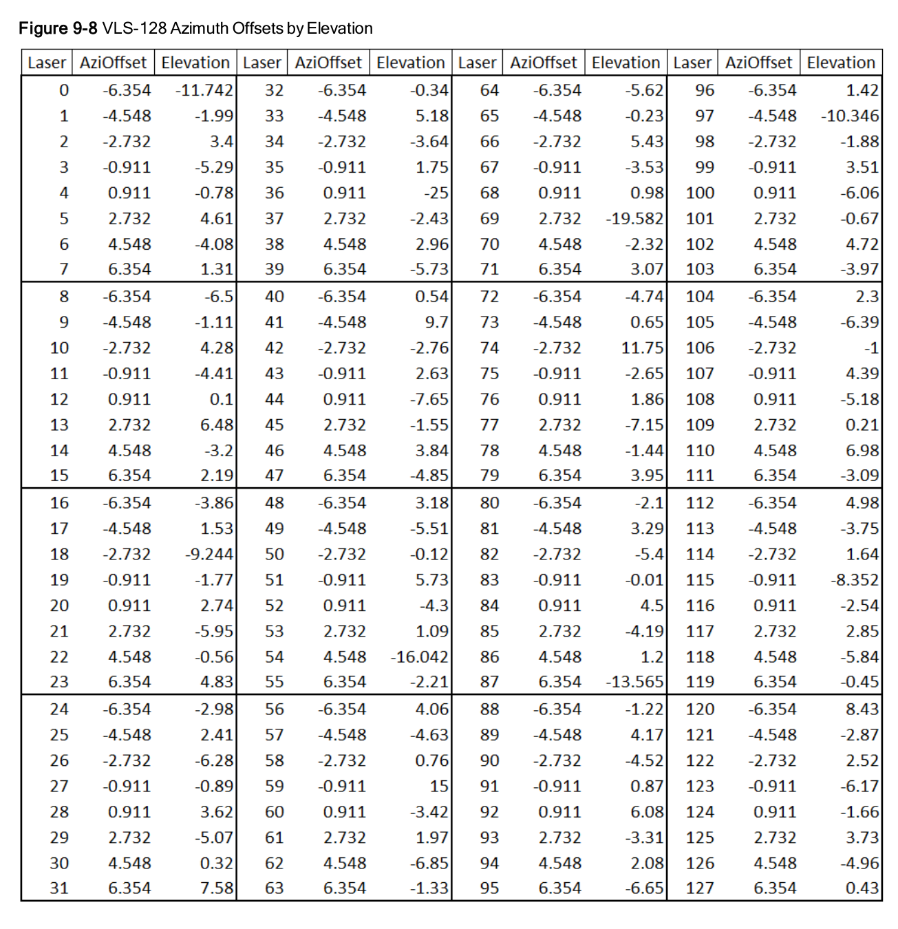
Figure 9-8 from the exact Alpha Prime/VLS-128 user manual, page 65.#

The resulting azimuth and elevation arrays each contain 128 values. Elevation spans -25 to +15 degrees, and the first azimuth group is [-6.354, -4.548, -2.732, -0.911, 0.911, 2.732, 4.548, 6.354].

The user manual uses zero-based channel IDs 0 through 127, while the generic Lidar core input uses one-based authored channelId values 1 through 128. Manual channel ID n is therefore authored as channelId n + 1. The core normalizes the authored value at runtime, so PointCloud ChannelId output n maps directly to manual channel ID and figure laser ID n. All emitters use rangeId = 0, which selects the single 0.3-300 m range region authored by the profile.

Derive the Firing Times#

The manual provides more than a point rate: it gives the firing sequence and the maintenance gaps.

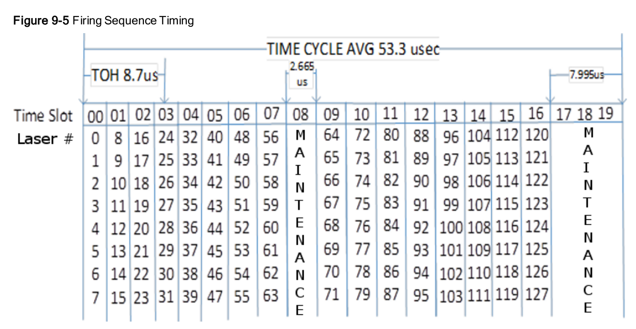
Figure 9-5 from the exact Alpha Prime/VLS-128 user manual, page 63.#

For the zero-based laser ID i used by Figure 9-5, integer division gives the firing group:

firing_group_index = (i // 8) + (i // 64)
fire_time_ns = 2665 * firing_group_index

The i // 64 term inserts the first 2.665 us maintenance interval before laser IDs and manual channel IDs 64-71. The resulting fireTimeNs values run from 0 through 42,640 ns. The 53.3 us tick period includes the remaining maintenance time after the last group.

The manual’s -8.7 us adjustment aligns a data point with the top-of-hour timestamp stored in a physical UDP packet. It is not added to fireTimeNs because the simulation array stores a non-negative delta from the model’s firing-pattern tick. Apply packet timestamp conventions in an encoder or downstream packet comparison, not by making the emitter times negative.

Configure Range and Returns#

float omni:sensor:Core:nearRangeM = 0.3
float omni:sensor:Core:farRangeM = 300.0
float omni:sensor:Core:rangeResolutionM = 0.004
float omni:sensor:Core:rangeAccuracyM = 0.03
float omni:sensor:Core:minReflectance = 0.10
float omni:sensor:Core:minReflectionRangeM = 300.0
uint omni:sensor:Core:maxReturns = 2
float omni:sensor:Core:minDistBetweenEchosM = 1.0
uint omni:sensor:Core:rangeCount = 1
float[] omni:sensor:Core:rangesMinM = [0.3]
float[] omni:sensor:Core:rangesMaxM = [300.0]

farRangeM, rangeResolutionM, maxReturns, and minDistBetweenEchosM map directly to published behavior. nearRangeM does not: neither source publishes a minimum range, so 0.3 m is the generic model’s initial value and must be checked against hardware.

The 4 mm value is the resolution of the physical packet’s integer distance field. It is available to packet encoders, but raw generic-model point-cloud coordinates are not necessarily quantized to 4 mm. Do not use it as a quantization requirement for the internal floating-point point-cloud output.

The datasheet’s +/-3 cm claim is typical wall-test accuracy across most channels and varies with range, temperature, and reflectivity. rangeAccuracyM controls a distance-dependent Gaussian uncertainty in the generic model, so 0.03 is an initial approximation, not an exact translation of a hard bound.

The generic model has only one reflectance/range threshold anchor, so this profile uses the farther 10%/300 m detection point. Keep the published 5%/180 m point as an independent validation check; the selected intensity processing and radiometric model mean that either anchor does not automatically guarantee the other.

Configure Beam and Intensity Behavior#

The manual publishes both divergence axes precisely.

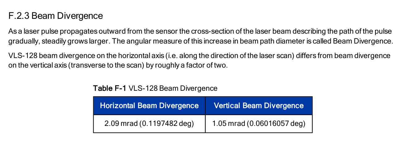
Table F-1 from the exact Alpha Prime/VLS-128 user manual, page 117.#

token omni:sensor:Core:rayType = "IDEALIZED"
float omni:sensor:Core:divergenceHorDeg = 0.1197482
float omni:sensor:Core:divergenceVerDeg = 0.06016057
float omni:sensor:Core:waveLengthNm = 905.0

The divergence values participate in radiometric threshold and intensity calculations even with the default, single-ray IDEALIZED type. The manual depicts the real spot as a rectangular pattern made of three bands, which none of the available idealized, Gaussian, or uniform representations reproduces exactly. Start with IDEALIZED. GAUSSIAN_BEAM traces multiple rays to represent a geometric footprint, has a substantial performance cost, and should be enabled only when higher-fidelity footprint and partial-hit behavior is required and validated against measurements.

The manual says calibrated reflectivity is intended to be independent of distance and laser power, with diffuse values in the lower part of the 0-255 range and retroreflectors in the upper part. The closest public-data starting configuration is:

token omni:sensor:Core:intensityProcessing = "NORMALIZATION"
token omni:sensor:Core:intensityMappingType = "LINEAR"
float omni:sensor:Core:intensityScalePercent = 255.0

NORMALIZATION is the preferred generic starting mode and matches the output scale, but not Velodyne’s proprietary calibration curve or the diffuse/retroreflector transition. Use CORRECTION only when calibration data shows that its range-dependent correction better represents the target sensor. peakPowerW, pulseTimeNs, detector properties, and multi-return power fractions are not published in these documents. The asset retains generic-model starting values for the required radiometric calculation and labels them as calibration inputs.

What Is Mappable and What Still Needs Work#

Easily Mappable or Uniquely Derivable#

The following information can be taken from the two public documents without hardware measurement:

Rotary scan type, clockwise market-frame azimuth, full horizontal field of view, and mounting/data-origin convention.
Frame-rate range and the coupled angular firing resolution at each supported RPM.
Number of channels and emitters, zero-based manual and output channel IDs, corresponding one-based authored channel IDs, all elevation angles, and all azimuth offsets.
Intra-sequence firing times, group-of-eight structure, and maintenance gaps.
Maximum range, packet distance resolution, typical accuracy value, and the two published reflectance/range detection points.
Return capacity and minimum separation for dual returns.
Beam divergence, nominal wavelength for the selected product revision, reflectivity output scale, and candidate point rate.

Published but Not One-to-One#

These values are available, but the generic model cannot represent the claim exactly with one attribute:

Published behavior	Model limitation	Recommended treatment
Detection at 5%/180 m and 10%/300 m	One `minReflectance`/`minReflectionRangeM` anchor	Use 10%/300 m as the profile anchor to preserve the published far-range detection point, and keep 5%/180 m as a validation point.
Typical +/-3 cm accuracy	`rangeAccuracyM` is a distance-dependent Gaussian scale	Start at 0.03 m and fit the simulated residual distribution to wall-test data by distance, channel, reflectivity, and temperature.
Three-band rectangular laser spot	Available ray types are idealized, Gaussian, or uniform	Start with `IDEALIZED` and use `GAUSSIAN_BEAM` only when higher-fidelity footprint behavior is needed and its performance cost is acceptable.
Calibrated 0-255 reflectivity with diffuse/retro ranges	A linear mapping does not reproduce the proprietary transfer function	Fit encoding/decoding curves from NIST reflectance panels and retroreflectors at multiple ranges.
Strongest, last, and dual return modes	`maxReturns` sets capacity but does not by itself reproduce every firmware selection rule	If two returns do not expose enough candidates for the desired selection, increase `maxReturns` and select strongest, last, or dual returns in post-processing.

Not Published and Requiring Calibration#

These model inputs cannot be recovered from the two public PDFs:

Attribute or behavior	Why the source is insufficient	Useful calibration experiment
`nearRangeM` and any near-field blind zone	Only maximum/detection ranges are published	Move a diffuse target through the near field and record first reliable detection by channel.
`peakPowerW`, `pulseTimeNs`, `focusDistM`, `Msquared`, and beam waist	Laser class, wavelength, and divergence do not uniquely determine these values	Use optical characterization if available; otherwise fit intensity and close-echo behavior without claiming physical laser power.
Detector aperture, quantum efficiency, pixel pitch, bit depth, and calibration gain	No detector transfer characteristics are published	Fit returned intensity against calibrated reflectance targets over range and incidence angle.
Angular noise distributions	Nominal angles are published, but random and temperature-dependent error are not	Fit per-channel angular residuals from large planar targets. Keep synthetic jitter at zero until measured.
Per-unit angle, origin, and distance corrections	Figure 9-8 is a nominal model table, not a serial-number calibration	Import unit-specific calibration when available or estimate channel residuals from a controlled target survey.
Reflection/transmission power split for multiple returns	The manual describes causes and selection rules, not an energy split	Use layered vegetation, mesh, glass, and partial-occlusion targets and compare echo intensity/order.
Full intensity encoding curve	The diffuse and retroreflector ranges are described, but no transfer curve is published	Capture 0-100% NIST targets plus retroreflectors at several distances and fit a non-linear mapping.
Interference mitigation and adverse-weather detection probability	Product capability is stated without an exposed algorithm or probability model	Treat interference and atmospheric models as separate validated effects using controlled multi-sensor and weather data.

Published but Outside the Generic Lidar Core#

Power consumption, supply voltage, weight, enclosure dimensions, IP67 protection, operating/storage temperature, Ethernet packet transport, GPS/NMEA input, and proprietary sensor-to-sensor interference mitigation are useful integration requirements but do not map to generic Lidar core attributes. Represent physical dimensions in mounting, visual, and collision assets. This profile represents the 66.11 mm data-origin offset with the emitters’ vertOffsetM values; do not apply the same offset again in the mounting transform. Represent environment, networking, synchronization, and power behavior in their corresponding simulation systems rather than inventing Lidar parameters.

Use the Asset#

Download Velodyne_Alpha_Prime_Rev4.usda and place it beside the scene that will use it. Reference the profile’s default prim instead of copying its attributes into every scenario. For example, a parent scene can include and position the sensor as follows:

#usda 1.0
(
    defaultPrim = "World"
    metersPerUnit = 1
    upAxis = "Z"
)

def Xform "World"
{
    def Xform "Sensors"
    {
        over "AlphaPrime" (
            prepend references = @./Velodyne_Alpha_Prime_Rev4.usda@
        )
        {
            double3 xformOp:translate = (0, 0, 2)
            uniform token[] xformOpOrder = ["xformOp:translate"]
        }
    }
}

The untyped over preserves the referenced prim’s OmniLidar type. The reference uses the asset’s declared defaultPrim, so no internal prim path is required. The asset exposes both GenericModelOutput and PointCloud for convenience. Applications typically retain one format, remove the unused render variable from orderedVars, and request only the channels they need.

Place the referenced prim at the real sensor’s mechanical base. The profile’s emitter origins are offset by 0.06611 m along the sensor’s +Z axis to represent the published data origin.

For moving sensors or moving targets, enable renderer Motion BVH and choose the required output motion-compensation state as described in Omniverse Lidar Extension.

Validate the Asset#

Checker Preflight#

Before launching a rendered simulation, validate the downloaded file with the sensor checker utility. Run this in the Kit Sensors app, or another Kit app that enables omni.sensors.nv.common and exposes its bundled sensor_checker Python module:

import sensor_checker as sc

asset_path = "/path/to/Velodyne_Alpha_Prime_Rev4.usda"
prim_path = "/Velodyne_Alpha_Prime_Rev4"

model = sc.ModelInfo()
model.modelName = "lidar.core"
model.modelVersion = "1.0"
model.schemaVersion = "1.0"
model.modelVendor = "nv"
model.marketName = "Velodyne Alpha Prime Rev 4 (VLS-128)"

checker = sc.SensorCheckerUtil()
error = checker.init(model)
if error:
    raise RuntimeError(f"Failed to initialize the Lidar checker: {error}")

error = checker.validateParams(asset_path, prim_path)
if error:
    raise ValueError(f"Invalid Lidar parameters: {error}")

schedule = checker.getSchedulerInfo()
if schedule.errorString:
    raise ValueError(f"Invalid Lidar schedule: {schedule.errorString}")

print("Alpha Prime Lidar parameters and schedule are valid")

ModelInfo selects the generic Lidar checker implementation; it does not replace the product metadata authored in the USDA file. validateParams checks required attributes, types, ranges, and array consistency, while getSchedulerInfo verifies that the firing pattern produces a valid schedule.

Geometry and Timing Checks#

Use a simple scene before a vehicle-scale environment:

Check	Test setup	Expected result
Coordinate orientation	Put narrow targets on +Y and +X and inspect the first scan sector	Tick zero is centered on +Y and the scan proceeds clockwise toward +X.
Channel pattern	Put a large vertical wall around the sensor and plot elevation by `ChannelId`	PointCloud `ChannelId` values 0-127 map directly to manual channel IDs and Figure 9-8 laser IDs 0-127 and span -25 to +15 degrees non-linearly.
Full rotation rate	Run with a stable simulation clock for several seconds	Ten complete rotations per second at the selected 600 RPM configuration.
Firing rate	Count candidate rays/ticks before scene filtering	Every rotation contains 1876 ticks, giving 18,760 ticks and 2,401,280 single-return candidates per second. The exact manual-derived cadence is 18,761.726 Hz before scheduler quantization.
Intra-tick time	Inspect `TimeOffsetNs` grouped by channel	Groups of eight share fire times; output `ChannelId` 64, corresponding to Figure 9-5 laser ID and manual channel ID 64, starts at 23,985 ns after the maintenance gap.

Range, Intensity, and Return Checks#

Use flat targets whose geometry, reflectivity, and separation are known:

Place diffuse walls at several known distances and compare mean range and residual standard deviation per channel. Do not treat the datasheet’s typical +/-3 cm statement as a guaranteed Gaussian sigma.
Verify that returns beyond 300 m are rejected. Determine the real near-field cutoff separately and replace the 0.3 m starting value.
Use a 10% NIST-equivalent material at 300 m to validate the selected threshold anchor. Also verify the published 5%/180 m point without weakening the required 10%/300 m detection behavior.
Place two partially visible surfaces less than and greater than 1 m apart. Dual-return output should not resolve the closer pair and can report two echoes for the separated pair when the material/geometry permits both paths.
Compare diffuse and retroreflective targets over distance. Fit a non-linear intensity mapping only after collecting enough points to reproduce the real 0-255 distribution.

Compare with Real Sensor Data#

For a high-fidelity profile, record a stationary Alpha Prime at 600 RPM in strongest, last, and dual-return modes. Use surveyed planar targets at multiple distances and reflectances, then compare simulation and capture directly by zero-based ChannelId; the one-based conversion applies only to the authored generic-core input:

detection probability and dropout rate;
range bias and spread;
elevation and azimuth residuals;
intensity distribution;
echo count, ordering, and separation;
timing within a rotation.

Tune only the parameters identified as approximations or calibration inputs. Keep the directly sourced geometry and timing fixed unless unit-specific calibration demonstrates a real difference. This separation prevents a radiometric mismatch from being hidden by changing the documented scan pattern.

Result and Limitations#

The completed asset reproduces the public nominal scan geometry, firing schedule, range envelope, return capacity, echo separation, beam divergence, and output scale of the Alpha Prime/VLS-128 source set. Its remaining uncertainty is explicit: minimum range, beam shape beyond divergence, laser/detector radiometry, proprietary reflectivity calibration, per-unit corrections, angular-noise distributions, and firmware-specific return selection require measured data.

That is the practical boundary of spec-sheet parameterization. Missing public information is a calibration task; published information with different model semantics is an approximation task; environmental or electrical information with no Lidar-core attribute belongs in another simulation subsystem.