Lidar Parameterization Tutorial: Blickfeld Cube 1

This tutorial builds a working OmniLidar profile for the Blickfeld Cube 1 from public manufacturer documentation. Unlike the rotary Velodyne Alpha Prime tutorial and the rotary or explicit-frame SICK TiM781 tutorial, the Cube 1 uses two resonant MEMS mirrors to draw a configurable Lissajous pattern.

No captured Cube 1 frame is available for this example. The firing pattern is therefore calculated from the equations published in the Blickfeld software manual. The completed Blickfeld_Cube1_Analytic.usda profile and its generator are documentation-derived analytic starting points, not a captured factory preset or a certified digital twin.

Important

Treat the resulting USDA as a deliberately vanilla, documentation-derived baseline. It contains what can be copied or reasonably inferred from the public manuals. Emitter and detector behavior that those sources do not define–including unit-specific optical power, receiver response and thresholds, noise, corrections, and intensity transfer–remains generic or approximate and must be tuned against measured sensor data for higher-fidelity use.

Source Documents

This tutorial uses these Blickfeld sources:

• Cube 1 Datasheet v2.1, document v2.1-EN-#42369-IH, published in 2022 for firmware v1.25.10.

• Blickfeld scan-pattern documentation, from the Blickfeld Software Manual v1.6.20, accessed July 27, 2026.

• Blickfeld protocol definitions, Blickfeld-Scanner-Library v2.20.6, accessed July 27, 2026.

The datasheet defines the Cube 1 product envelope. The scan-pattern page supplies the mirror equations, the definition of a scanline, the relationship between frame duration and line count, the exemplary ramp, and the observed line order. The protocol definitions distinguish configurable pulse modes and describe the fields available in a captured point-cloud frame.

The revisions are not one matched source set: the 2022 datasheet targets firmware v1.25.10, while the current software manual and protocol documentation are newer. Recheck the constraints reported by the target device before copying this profile into a production configuration.

Interpreting Source Confidence

Each mapping below belongs to one of four categories:

Category	Meaning	How to use it
Direct	Source and simulation values have the same physical meaning and units.	Copy the value, then verify coordinate, boundary, and array conventions.
Derived	The source provides enough information to calculate the value.	Preserve the equation and every selected source assumption.
Approximation	A published claim exists, but the generic core uses different semantics.	Use it as an initial condition and validate it against measurements.
Calibration	Public sources do not define the value or the exact device behavior.	Retain a documented generic starting value and replace it with measured data.

Read the Product-Level Specifications

The datasheet provides range, angular envelope, configurable resolution, and conditional accuracy claims.

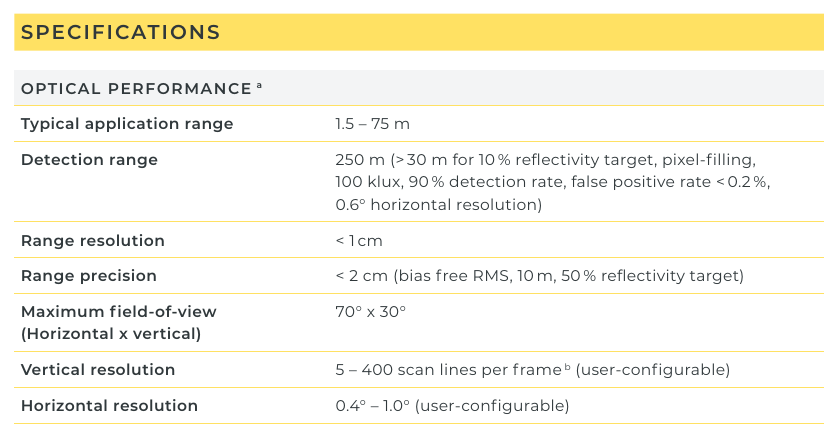
Excerpt from the Cube 1 Datasheet v2.1, page 1.

It separately describes scan cadence, returns, laser properties, and output fields.

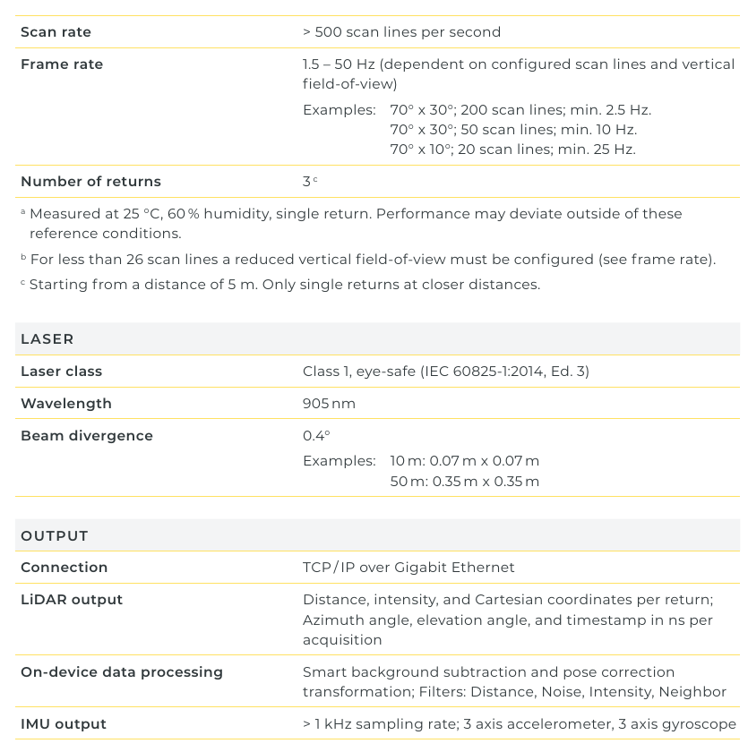
Excerpt from the Cube 1 Datasheet v2.1, page 1.

The source-to-model mapping used by this example is:

Manufacturer information	Simulation attribute or action	Value in this profile	Category	Notes
Two resonant MEMS mirrors and software-defined pattern	scanType and explicit emitter arrays	SOLID_STATE	Direct mechanism, derived schedule	Every virtual emitter is one analytically derived pulse opportunity.
Maximum 70 x 30 degree field of view	Analytic mirror envelope	70 x 30 degrees nominal	Direct envelope	The discrete pulse grid does not fire exactly at the turning points.
5-400 scanlines per frame	numLines	50	Direct datasheet example	The datasheet pairs 50 lines with a 70 x 30 degree field of view and a minimum 10 Hz frame rate.
0.4-1.0 degree horizontal resolution	Explicit horizontal grid	0.6 degrees	Selected within range	This is also the resolution in the datasheet’s conditional 10% target claim.
More than 500 scanlines per second	Analytic mirror frequency	250 Hz, giving a nominal 500 lines/s	Derived approximation	This follows the rounded 50-line, 10 Hz datasheet example; it is not a measured eigenfrequency.
1.5-50 Hz frame rate	tickRate, scanRateBaseHz, patternFiringRateHz	10, 10, 10	Selected lower bound	The renderer and model schedules apply one firing pattern per complete 10 Hz scan.
Typical application range 1.5-75 m	nearRangeM and validation range	1.5 m near limit; validate through 75 m	Approximation	The source does not call 1.5 m a hard minimum.
Detection range 250 m	farRangeM	250 m	Approximation	Target reflectivity and other conditions are not stated for the 250 m limit.
More than 30 m on a 10% target under stated conditions	minReflectance, minReflectionRangeM	0.10, 30 m	Approximation	This is a conservative generic threshold anchor, not a reproduction of detection probability.
Range resolution below 1 cm	rangeResolutionM	0.01 m	Conservative approximation	The published bound does not provide an exact reporting increment.
Bias-free RMS precision below 2 cm at 10 m and 50% reflectivity	rangeAccuracyM	0.02 m	Approximation	The generic error grows with range and does not encode the source conditions.
905 nm wavelength	waveLengthNm	905 nm	Direct	Used by the material and radiometric model.
0.4 degree beam divergence	divergenceHorDeg, divergenceVerDeg	0.4, 0.4 degrees	Direct	The square 7 cm and 35 cm spot examples at 10 m and 50 m support both axes.
Up to three returns, one below 5 m	maxReturns	3	Partly direct	The generic global capacity cannot reduce the limit to one below 5 m.
Distance, intensity, Cartesian position, angles, and nanosecond timestamp	PointCloud channels	Requested as needed	Direct output concepts	Blickfeld’s exact encoding, selection, and intensity transfer remain separate.

Select an Analytic Reference Pattern

Cube 1 does not have one immutable firing pattern. The device exposes horizontal and vertical field of view, up-ramp and down-ramp line counts, pulse mode, and related constraints. An exact profile normally starts with one recorded point-cloud frame and the active scan-pattern configuration.

Without that data, this tutorial deliberately selects one reproducible point inside the published envelope:

Choice	Value	Reason
Nominal field-of-view envelope	70 x 30 degrees	Maximum Cube 1 envelope from the datasheet.
Mirror frequency	250 Hz	Derived from 50 lines, 10 Hz, and the published line-count equation.
Scanlines	50	Matches the datasheet’s 70 x 30 degree, minimum 10 Hz example.
Ramp	Continuous 3:1 duration ratio	Follows the published exemplary function; its peak occurs 37.5 scanlines into this frame.
Horizontal spacing	0.6 degrees	Within the configurable range and used by one datasheet detection claim.
Pulse-grid behavior	Same grid on every line	Corresponds to EQUI_HORIZONTAL_ANGLE rather than undocumented interleave edge behavior.
Capture mode	Full-period, scan-aligned	Matches one explicit solid-state frame with accumulateOutputs = true.

This is not claimed to be a named WebGUI preset. In particular, the protocol documents INTERLEAVE as the default pulse type and describes a quarter-spacing shift between alternating scanlines. It does not define the sign of that shift, the initial grid phase, or the edge-rounding rule. The profile therefore uses the simpler documented equal-horizontal-angle behavior and leaves interleaving for validation against a captured frame.

Build the Profile

Start with an OmniLidar prim and apply the generic core API:

def OmniLidar "Blickfeld_Cube1_Analytic" (
    prepend apiSchemas = ["OmniSensorGenericLidarCoreAPI"]
)
{
    string omni:sensor:modelName = "LidarCore"
    string omni:sensor:modelVersion = "0.0.0"
    string omni:sensor:modelVendor = "NVIDIA"
    string omni:sensor:marketName = "Blickfeld Cube 1"
    float omni:sensor:tickRate = 10.0
    uint omni:sensor:Core:scanRateBaseHz = 10
    uint omni:sensor:Core:patternFiringRateHz = 10

    token omni:sensor:Core:scanType = "SOLID_STATE"
    bool omni:sensor:Core:accumulateOutputs = true
}

tickRate controls how often Kit schedules the sensor, and the complete modeled scan rate is authored with scanRateBaseHz. For this solid-state profile, set patternFiringRateHz to the same value so one explicit firing pattern is applied per scheduled scan. Rotary-only attributes such as rotationDirection do not participate in this schedule.

Derive Frame Duration and Line Rate

Blickfeld defines one scanline as one half-period of the horizontal mirror. For mirror frequency \(f\), frame duration \(T\), and line count \(N\):

\[N = 2 T f\]

For the selected 50 lines and 10 Hz frame rate:

T = 1 / 10 Hz = 0.1 s
line_rate = 50 / 0.1 s = 500 lines/s
f = 50 / (2 * 0.1 s) = 250 Hz

This reproduces the rounded arithmetic of the datasheet’s 50-line, minimum 10 Hz example. The separate >500 scanlines/s statement indicates that a real device may run slightly faster; 250 Hz is a derived analytic value, not a measured Cube 1 eigenfrequency. The profile contains 5,850 candidate ray slots per frame and therefore 58,500 candidate ray slots per second. That number is a result of this analytic selection, not a published Cube 1 point-rate specification.

The scan-pattern page contains inconsistent example prose. It describes a frame as one mirror period, but also defines \(N=2Tf\) and calls 40 scanlines 20 periods. Its printed \(T=2/f\) for that example would produce four rather than 40 lines. This tutorial follows the scanline definition and \(N=2Tf\). For its selected 50-line frame, that gives \(T=25/f\).

Use the Published Mirror Functions

The public page describes a 1:1 Lissajous pattern with horizontal and vertical functions:

\[\theta_H(t) = \frac{H}{2}\cos(2\pi f t)\]

\[\theta_V(t) = r(t)\frac{V}{2}\sin(2\pi f t)\]

where \(H\) and \(V\) are the nominal horizontal and vertical field-of-view envelopes. The exemplary ramp is:

\[\begin{split}r(t) = \begin{cases} \frac{4t}{3T}, & 0 \leq t \leq \frac{3T}{4} \\ 4-\frac{4t}{T}, & \frac{3T}{4} < t \leq T \end{cases}\end{split}\]

The published plot makes the unequal ramp durations visible.

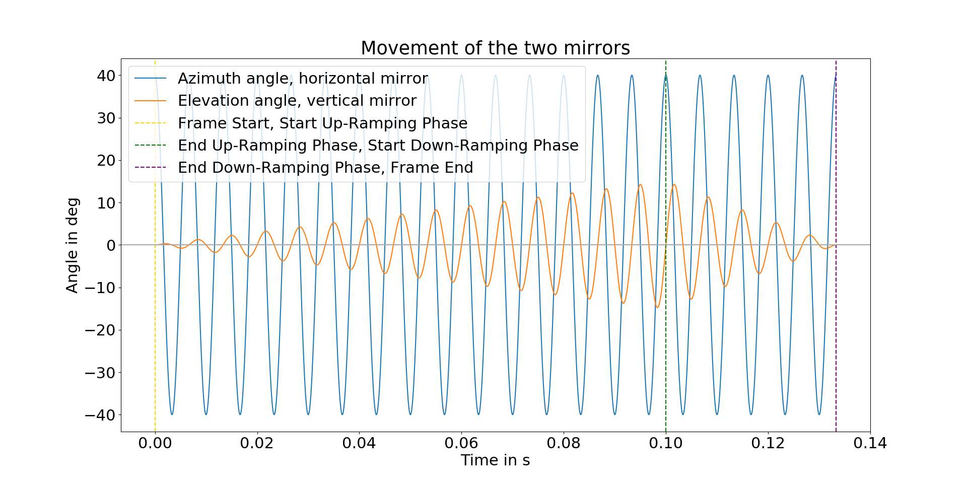
Figure 1 from the Blickfeld scan-pattern documentation. Its values illustrate the mechanism and are not all Cube 1 profile values.

The ramp reaches one at three quarters of the frame. For 50 scanlines, that transition occurs 37.5 scanlines into the frame, halfway through scanline 37 when numbered from zero. The continuous analytic trajectory is well-defined, but it cannot be described as integer up-ramp and down-ramp line counts. The actual Cube 1 split for the datasheet example is not published. The prose on the same page calls these two halves; the formula and plot are unambiguously 3:1, so the generator follows the formula.

The page also states a \(\pi/4\) mirror phase difference, while the shown cosine and sine equations imply \(\pi/2\). The profile follows the explicit equations and the documented line order. An exact device fit must replace this analytic interpretation with captured directions and timestamps.

Sample Horizontal Angle, Not Uniform Time

A 0.6-degree grid cannot include both exact 70-degree endpoints symmetrically: 70 / 0.6 is not an integer. The profile centers 117 directions inside the envelope:

x[j] = -34.8 + 0.6 * j degrees,  j = 0..116

This gives 116 exact 0.6-degree intervals, 69.6 degrees of sampled horizontal coverage, and a 0.2-degree margin to each mirror turnaround. Omitting the exact turning points also prevents adjacent scanlines from sharing one timestamp.

The mirror moves slowly near a turnaround and fastest at the center. Uniform fireTimeNs increments would therefore contradict the published sinusoid. For even line \(\ell=2k\), traverse \(x\) from +34.8 to -34.8:

\[t_{\ell}(x) = \frac{2\pi k + \arccos(x/35)}{2\pi f}\]

For odd line \(\ell=2k+1\), traverse \(x\) from -34.8 to +34.8:

\[t_{\ell}(x) = \frac{2\pi(k+1) - \arccos(x/35)}{2\pi f}\]

Calculate every value from absolute time and round once to nanoseconds. Do not accumulate already-rounded deltas. The resulting 5,850 times are strictly increasing:

Quantity	Analytic result
Rounded frame duration	100,000,000 ns
First pulse	68,090 ns
Last pulse	99,931,910 ns
Minimum adjacent pulse gap	10,914 ns
Gap across a mirror turnaround	Approximately 136,180 ns

Strict timestamp uniqueness is important to the current solid-state scheduler, which associates one emitter with each firing time.

Derive Vertical Angles and Coordinate Signs

The scan-pattern description says the first line starts near the center and moves from left to right while the vertical mirror moves toward the bottom. Later lines alternate direction and appear above, below, then farther above and below the first line.

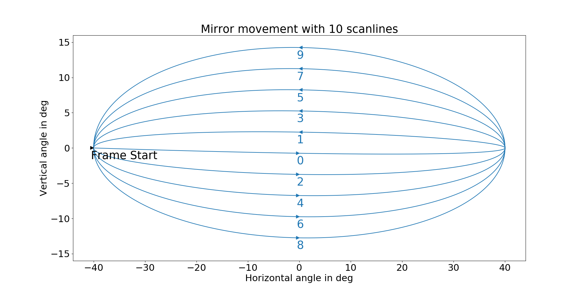
Figure 2 from the Blickfeld scan-pattern documentation. It uses a ten-line, 80-degree horizontal illustration rather than this Cube 1 profile.

This tutorial defines the core sensor frame as +X forward, +Y left, and +Z up. Positive physical azimuth is therefore toward sensor-left. For the first line, the analytic \(\theta_H\) moves from positive to negative, or left to right.

The solid-state core converts authored azimuth \(A\) to the physical direction \(-A\). The profile therefore authors:

azimuthDeg(t) = -theta_H(t)
elevationDeg(t) = -r(t) * 15 deg * sin(2*pi*250*t)

The vertical negation makes the first line move downward as described in the manual. It also resolves a sign conflict between the page’s equation, prose, and figure in one explicitly documented sensor frame. If recorded Blickfeld azimuth and elevation use a different market-frame sign, transform the captured directions once before replacing these arrays.

Although one pulse reaches the positive vertical extremum, the discrete pattern does not reach both nominal vertical limits. This profile’s authored elevations span approximately -14.600 to +15.000 degrees, or 29.600 degrees total. Do not report 70 x 30 degrees as the exact discrete point bounds.

Author the Solid-State Arrays

The profile has one emitter entry for every line and horizontal direction:

uint omni:sensor:Core:numberOfEmitters = 5850
uint omni:sensor:Core:numberOfChannels = 5850
uint omni:sensor:Core:numLines = 50
uint[] omni:sensor:Core:numRaysPerLine = [
    117, 117, 117, 117, 117, 117, 117, 117, 117, 117,
    117, 117, 117, 117, 117, 117, 117, 117, 117, 117,
    117, 117, 117, 117, 117, 117, 117, 117, 117, 117,
    117, 117, 117, 117, 117, 117, 117, 117, 117, 117,
    117, 117, 117, 117, 117, 117, 117, 117, 117, 117
]

The current solid-state implementation uses numberOfChannels as output capacity indexed by emitter ID. This profile therefore makes it equal the 5,850 emitter slots. Independently of that storage requirement, it uses the complete one-based range for channel IDs. This is an analytic indexing convention, not a claim that Cube 1 has 5,850 physical detector channels.

Public documentation does not assign device channel IDs to the pulse slots. This analytic profile assigns one distinct channel ID to every virtual emitter:

uint[] omni:sensor:Core:emitterState:s001:channelId = [1, 2, ..., 5850]

Authored channelId covers the required one-based range from 1 through numberOfChannels, so PointCloud ChannelId covers 0 through 5,849. PointCloud EmitterId identifies the same 0-5,849 analytic ray slots. The resulting one-to-one channel mapping is redundant with EmitterId but keeps the authored channel range explicit. bank contains 117 copies of each zero-based line number from 0 through 49. All rays select range region zero.

Configure Range and Error

float omni:sensor:Core:nearRangeM = 1.5
float omni:sensor:Core:farRangeM = 250.0
float omni:sensor:Core:rangeResolutionM = 0.01
float omni:sensor:Core:rangeAccuracyM = 0.02
float omni:sensor:Core:minReflectance = 0.10
float omni:sensor:Core:minReflectionRangeM = 30.0
uint omni:sensor:Core:rangeCount = 1
float[] omni:sensor:Core:rangesMinM = [1.5]
float[] omni:sensor:Core:rangesMaxM = [250.0]

These attributes make conditional product claims into the generic core’s required scalar parameters, so none is a perfect one-to-one mapping.

The lower end of the typical application range is used as an approximate near limit, not asserted as the physical minimum range. The 250 m detection claim does not state a target and is not the typical 75 m application limit. The 10% result is stated as more than 30 m for a pixel-filling target at 100 klux, 90% detection rate, false-positive rate below 0.2%, and 0.6-degree horizontal resolution. Using 30 m as one generic threshold anchor is conservative but does not encode those probabilities or conditions.

Likewise, 0.01 and 0.02 conservatively represent published < 1 cm and < 2 cm bounds. The internal floating-point PointCloud is not required to quantize every coordinate to 1 cm. Fit range bias and residual spread across distance, reflectivity, incidence angle, illumination, and temperature before claiming range fidelity.

Configure Beam, Intensity, and Returns

token omni:sensor:Core:rayType = "IDEALIZED"
float omni:sensor:Core:waveLengthNm = 905.0
float omni:sensor:Core:divergenceHorDeg = 0.4
float omni:sensor:Core:divergenceVerDeg = 0.4
token omni:sensor:Core:intensityProcessing = "NORMALIZATION"
token omni:sensor:Core:intensityMappingType = "LINEAR"
uint omni:sensor:Core:maxReturns = 3

The divergence participates in radiometric behavior with IDEALIZED. Start with this lower-cost ray type. Use GAUSSIAN_BEAM only when partial-beam hits and geometric footprint fidelity are needed and validated, because it has a substantial ray-tracing cost.

The source publishes intensity as an output field but no radiometric transfer curve, scale, optical peak power, pulse duration, detector aperture, quantum efficiency, or calibration gain. NORMALIZATION with a linear map is therefore only a generic starting behavior. The profile inherits generic-core starting values for the unpublished radiometric inputs; replace them together from calibration rather than treating them as Cube 1 specifications.

maxReturns = 3 provides the published maximum capacity. It does not implement the device’s one-return restriction below 5 m, its return-selection policy, or the protocol’s return ordering. Implement those behaviors in a device-specific encoder or post-processing if they matter to the application.

What Is Mappable and What Still Needs Work

Easily Mappable or Uniquely Derivable

The public sources support:

• the solid-state mechanism and nominal maximum angular envelope;

• configured line count and horizontal spacing;

• line rate, derived 250 Hz mirror frequency, and nonuniform firing times once the datasheet’s 50-line, 10 Hz example and public equations are selected;

• the published exemplary 3:1 ramp;

• wavelength, divergence, and maximum return capacity;

• the output field concepts and source-based range validation points.

Published but Not One-to-One

Published behavior	Model or source limitation	Recommended treatment
Configurable scan pattern	This profile fixes one analytic selection	Regenerate arrays whenever field of view, spacing, line count, ramp, pulse mode, or device frequency changes.
Default interleaving	Shift sign, starting phase, and edge rules are not public	Use equal-horizontal-angle sampling until one real frame establishes the exact grid.
70 x 30 degree maximum field of view	Discrete pulses avoid the turnarounds and vertical extrema	Treat it as a nominal envelope; validate actual point bounds separately.
1.5-75 m typical range and 250 m detection range	Generic core requires one hard near/far interval	Use 1.5-250 m only as an operational starting interval and test the intended application range.
Conditional 10% target result	One threshold pair cannot encode detection probability and illumination	Use 10%/30 m as a conservative anchor and retain all source conditions in validation.
Below-bound range resolution and precision	Exact increment, distribution, and condition dependence are missing	Start with 0.01 m and 0.02 m, then fit reporting and error behavior independently.
Three returns, but one below 5 m	maxReturns is a global capacity	Apply the near-range restriction and return selection downstream if required.
Pose correction and filters	They are device post-processing rather than emitted-ray geometry	Compare raw uncompensated data, then reproduce selected processing in the perception pipeline.

Not Published and Requiring Calibration

The public sources do not uniquely define:

• the target device’s fixed mirror frequency and exact firmware ramp;

• scan-pattern acceleration limits, distortion correction, pulse-grid phase, or interleave boundary behavior;

• optical peak power, pulse duration, detector aperture and efficiency, echo separation, or the intensity transfer;

• the optical origin relative to the mechanical housing;

• per-unit angular and distance corrections or random-error distributions.

The profile places the prim at the assumed optical origin and authors no emitter-origin offsets. A housing or mounting asset must supply the measured optical transform.

Published but Outside the Generic Lidar Core

On-device background subtraction, pose correction, distance/noise/intensity/ neighbor filters, IMU transport, time synchronization, Ethernet protocol, power, enclosure, and environmental ratings do not become firing-pattern attributes.

For moving sensors or targets, enable renderer Motion BVH. NONCOMPENSATED is raw output with motion effects, similar to a real sensor’s uncompensated scan. COMPENSATED performs the motion-compensation step commonly applied near the beginning of perception stacks and is especially important for mapping.

Use the Asset

Reference the generated profile’s default prim:

#usda 1.0
(
    defaultPrim = "World"
    metersPerUnit = 1
    upAxis = "Z"
)

def Xform "World"
{
    over "Cube1" (
        prepend references = @./Blickfeld_Cube1_Analytic.usda@
    )
    {
        double3 xformOp:translate = (0, 0, 0.5)
        uniform token[] xformOpOrder = ["xformOp:translate"]
    }
}

The untyped over preserves the referenced OmniLidar type. The asset exposes GenericModelOutput and PointCloud for convenience. Applications typically retain one output, remove the unused render variable, and request only the channels they consume.

accumulateOutputs = true with a full-period, scan-aligned call represents one complete explicit frame. The current solid-state scheduler determines scan completion from inclusion of the final emitter rather than the exact nominal period boundary. Render-step partitions that end before the last firing time do not produce a complete scan.

After downloading the generator linked at the start of this tutorial, regenerate the profile with:

python3 generate_blickfeld_cube1_profile.py --output Blickfeld_Cube1_Analytic.usda

The generator validates the array lengths, timestamp order, and expected schedule endpoints before replacing the USDA file.

Validate the Asset

Checker Preflight

Run the sensor checker in the Kit Sensors app, or another Kit app that enables omni.sensors.nv.common and exposes its bundled sensor_checker module:

import sensor_checker as sc
from pxr import Usd

asset_path = "/path/to/Blickfeld_Cube1_Analytic.usda"
prim_path = "/Blickfeld_Cube1_Analytic"

model = sc.ModelInfo()
model.modelName = "lidar.core"
model.modelVersion = "1.0"
model.schemaVersion = "1.0"
model.modelVendor = "nv"
model.marketName = "Blickfeld Cube 1"

checker = sc.SensorCheckerUtil()
error = checker.init(model)
if error:
    raise RuntimeError(f"Failed to initialize the Lidar checker: {error}")

stage = Usd.Stage.Open(asset_path)
prim = stage.GetPrimAtPath(prim_path)
if not prim:
    raise ValueError(f"Missing Lidar prim {prim_path}")

error = checker.validateParams(prim)
if error:
    raise ValueError(f"Invalid Lidar parameters: {error}")

prefix = "omni:sensor:Core:"
emitters = prim.GetAttribute(prefix + "numberOfEmitters").Get()
channels = prim.GetAttribute(prefix + "numberOfChannels").Get()
lines = prim.GetAttribute(prefix + "numLines").Get()
rays = prim.GetAttribute(prefix + "numRaysPerLine").Get()
state = prefix + "emitterState:s001:"
fire = prim.GetAttribute(state + "fireTimeNs").Get()
channel = prim.GetAttribute(state + "channelId").Get()
bank = prim.GetAttribute(state + "bank").Get()

assert emitters == channels == 5850
assert lines == 50
assert list(rays) == [117] * 50
assert len(fire) == len(channel) == len(bank) == emitters
assert all(b > a for a, b in zip(fire, fire[1:]))
assert fire[0] == 68090
assert fire[-1] == 99931910
assert list(channel) == list(range(1, channels + 1))
assert list(bank) == [
    line for line in range(50) for _ in range(117)
]

print("Blickfeld Cube 1 analytic profile is structurally valid")

Geometry and Timing Checks

Use a simple static scene first:

Check	Test setup	Expected result
Coordinate orientation	Place narrow targets at center, left, right, above, and below	Line 0 moves left-to-right just below center; line 1 reverses just above center.
Frame and line cadence	Run with a stable simulation clock for several seconds	10 complete frames/s and 500 analytic scanlines/s.
Horizontal grid	Inspect output angles in a surrounding wall scene	117 directions per line, 0.6-degree increments, alternating direction, with sampled bounds +/-34.8 degrees.
Vertical pattern	Group PointCloud entries by bank or emitter range	The continuous ramp turns halfway through zero-based line 37; sampled elevation bounds are approximately -14.600 and +15.000 degrees.
Firing time	Inspect PointCloud TimeOffsetNs or authored fireTimeNs	Strictly increasing offsets from 68,090 through 99,931,910 ns, with larger gaps near turnarounds.
Point capacity	Use a surrounding static wall with one return	5,850 ray slots and at most 17,550 return slots.
Channel and emitter identity	Request ChannelId and EmitterId	Channel IDs and emitter IDs both cover 0-5,849.
Output completion	Compare ready status around the 100 ms period	A complete scan is available only after the final emitter is included.

Range, Beam, and Return Checks

Use surveyed, flat targets:

• Treat 1.5 m as an approximate operational cutoff and 75 m as the normal validation envelope, not as proven physical boundaries.

• Validate the separate 250 m detection claim with a target whose reflectivity, projected size, and illumination are recorded.

• Check a pixel-filling 10% target at 30 m and preserve the source’s illumination and probability conditions.

• Compare mean range bias and RMS residuals at 10 m on a 50% target before interpreting rangeAccuracyM = 0.02.

• Start small-object and edge tests with IDEALIZED. Evaluate GAUSSIAN_BEAM only if the 0.4-degree footprint needs a higher-fidelity geometric representation.

• Test layered targets both below and above 5 m. Add device-specific filtering if one near return and up to three farther returns are required.

• Fit intensity mapping from paired targets over range and incidence angle; the public documents do not define an intensity scale or curve.

Compare with Real Sensor Data

When a Cube 1 capture becomes available, record the active scan-pattern configuration and an unfiltered point-cloud frame. For every acquisition, retain scanline ID, azimuth, elevation, timestamp, return count, distance, and intensity. Use it to replace or confirm:

• the derived 250 Hz frequency and frame phase;

• the ramp, up/down line split, and nonlinear mirror distortion;

• horizontal grid phase, interleaving, edge inclusion, and line order;

• coordinate signs and optical origin;

• near-range return restriction and return selection;

• range error, dropout probability, beam-edge behavior, and intensity mapping.

Keep each directly sourced product limit separate from the selected analytic preset. That prevents a scan-pattern correction from being confused with radiometric calibration.

Result and Limitations

The completed profile is a deterministic solid-state encoding of one documentation-derived Cube 1 pattern. It follows the public mirror equations, uses a 70 x 30 degree nominal envelope, 50 scanlines at 10 Hz, 0.6-degree horizontal spacing, a continuous 3:1 ramp, and nonuniform inverse-cosine firing times.

Its remaining uncertainty is intentional and visible. The exact device frequency, ramp, pulse mode, distortion correction, optical origin, detector parameters, intensity mapping, and return policy require configuration data or a real capture. The sampled pattern covers 69.6 degrees horizontally and approximately 29.600 degrees vertically rather than firing at every nominal envelope extreme. Regenerate all dependent arrays together when any scan-pattern choice changes.