Example: Meshed Based Data

Import and Scale

• Launch Kit-CAE with the VTK extension as described in the first section.

• Click File > Open and browse to the directory containing the kitCAE_Sample.cgns file.

Note

Using File > Open is suitable for bringing data into a new stage, but if you have a stage already established and want to retain it, then use File > Import to bring in the data to the current session.

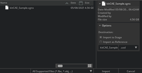
• Ensure the extensions in the dialog are set up either *.* or *.cgns and then select the file.

• Check Import to Stage (recommended) if you do not want to import as a reference.

• Click Import to import the dataset.

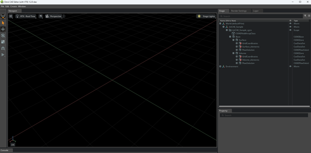
• View the Imported File

  Navigate to the Stage window and expand the nodes. You will see the file imported as shown below.

Note on Units

When importing data, no automatic unit conversion is performed. The data retains its original units. Kit-CAE uses centimeters (cm) as its default unit. If your imported data uses a different unit system, manually apply a transformation to ensure proper scaling.

In this example, the data is in meters (m) while the stage is in centimeters (cm). To scale the world properly:

• Select World.

• Go to Property > Transform and select Add Transforms.

• Click the icon to the right of Scale to sync the scale in all directions.

• Double-click on one of the directions (X, Y, or Z) or press Cntrl + C, and update the value from 1 to 100. Press Enter to apply the change.

• Add a rotation of -90 about the X axis.

This example includes data in two different datasets, Surface and Volume. A useful first step is to visualize the extent of each dataset using a bounding box.

Steps to Create a Bounding Box

Create a Bounding Box:

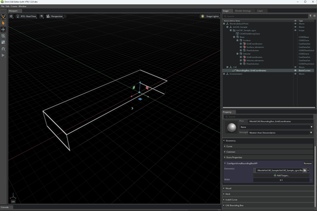
• In Stage/World/kitCAE_Sample_cgns/Base/Volume, right-click on GridCoordinate node to open the context menu.

• Navigate to, and select Create > CAE Algorithms > Bounding Box.

  • This creates a new prim named /CAE/BoundingBox_GridCoordinates.

Rename the Bounding Box (Optional):

You can rename the bounding box by double-clicking on the prim, or by selecting the prim and updating the name in the Property window.

Zoom into the Bounding Box:

To zoom into the bounding box, either zoom in interactively or press the shortcut key f, (Edit > Focus).

Adjust Bounding Box Properties:

In the Properties panel, you can change the width of the lines used for the bounding box by adjusting the Width attribute under CAE Bounding Box.

Note

A bounding box over multiple regions can be created by selecting Shift and selecting all regions of interest.

Create a Region of Interest

Setting a region of interest can be useful when working with NanoVDB data, as it can subset the domain to a smaller region of interest.

Create a Bounding Box for the Vehicle

• Repeat the steps above to create a bounding box for the Surface > GridCoordinates dataset.

• Rename this bounding box to Region of Interest.

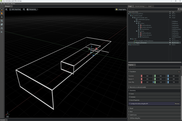
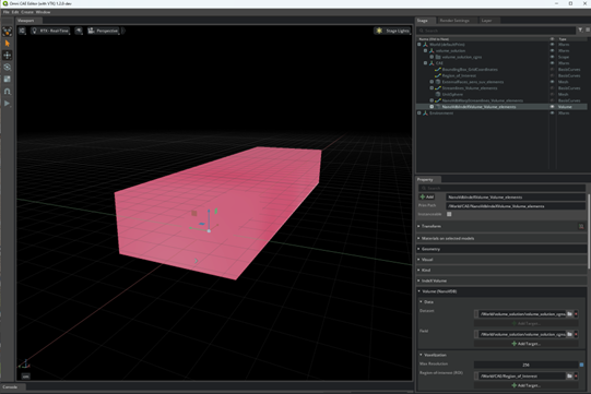
• Transform the Region of Interest to be slightly larger than the vehicle, encompassing the wake.

• Scale by X:2, Y:1, Z:1.

The Region of Interest will look like the following:

Visualizing Data with Points

A quick way to visualize what data is available in the dataset is by using points. Points create spheres at every vertex location in the dataset, providing a clear visualization of the dataset’s structure. In the next example we will visualize the surface of the car (aero_suv) by points.

• Hide the bounding box and region of interest created in the previous step.

Create Points

• Select the Surface_elements node in the Stage panel.

• Right-click on the node to return the context menu.

• Navigate to, and click on Create > CAE Algorithms > Points.

• Expand the newly created /CAE node and you will see Points_Surface_elements node under the expanded /CAE node.

View the Outline

An outline of the car should now be visible.

Adjust Point Properties

• Navigate to CAE/Points_Surface_elements/Property/CaeAlgorithmsPointsAPI.

• Next to Width change the value to 0.05.

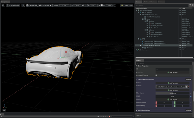
• Navigate to CAE/Points_Surface_elements/Property/CaeAlgorithmsPointsAPI and adjust the color of the points by specifying the field array. Click on the Add Target button next to Colors and select Wall_Shear_Stress_N_m2_mag under Surface/Flow_Solution, which is the wall shear stress magnitude.

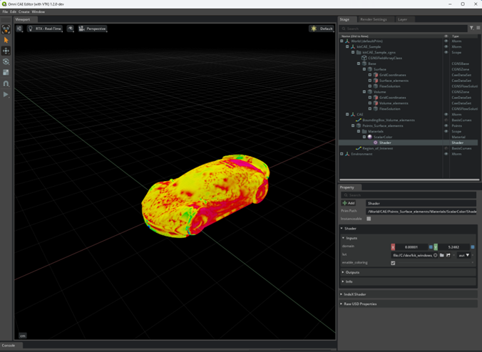
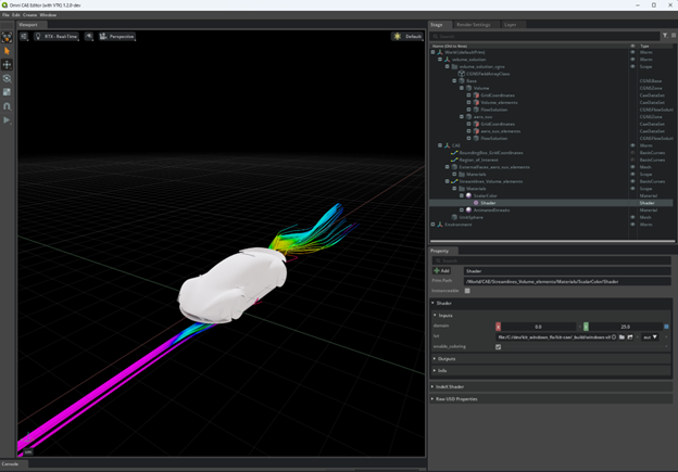
• Adjust the color by changing the domain min/max under Points_aero_suv_elements/Materials/ScalarColor/Shader.

• Under Inputs, the domain X and Y are the min/max of the color bar shown, specified at lut. The default color bar is called gist_rainbow, shown below.

The range is auto-loaded to the min and max range of the scalar data specified. The points should display as shown below.

The default width for the points used can be specified from the Render Settings panel. Set the renderer type to Real Time and then you should see a Points Default Width setting. If you are routinely opening large datasets, it is a good idea to set this setting to a small value like 0.01 by default. You can always override the width using the Width attribute on the Points prim as shown earlier.

Visualizing External Faces (VTK based)

External faces can be rendered to show a surface representation of the dataset if the connectivity of the cells is known. This is not possible for point-based datasets. Follow the steps below to visualize external faces for the Surface_elements dataset:

• Hide the Points_Surface_elements node created in the previous section.

• Fit the screen to view the new visualization clearly.

Create External Faces

• In Stage/World/kitCAE_Sample_cgns/Base/Surface, right-click on the Surface_elements node to open the context menu.

• Navigate to and select Create > CAE Algorithms > External Faces.

Expand the CAE Node

Expand the CAE node. You will see the ExternalFaces_Surface_elements node under the node.

Adjust Properties

In CAE/ExternalFaces_Surface_elements navigate to CaeAlgoritmsEcternalFacesAPI under Property.

Color Based on Scalar Quantity

To color the external faces based on a scalar quantity:

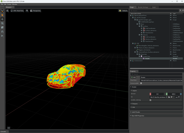
• Under Property/CaeAlgorithmsExternalFacesAPI/Colors, select Add Target and navigate to the simulation data of the car (Surface_elements/FlowSolution) and select Y_Plus.

• Adjust the min and max of the color bar under ExternalFaces_Surface_elements/Materials/ScalarColor/Shader, specifically under Shader/Inputs/domain.

• In the same section, ExternalFaces_Surface_elements/Materials/ScalarColor/Shader, lut is the color map of the scalar displayed.

Create Streamlines (VTK based)

Creating streamlines requires both a seed reference and a domain within the fluid domain to apply the streamlines. This example uses a UnitSphere as the seeding object.

Display car as solid color

Under Property/Shader of ExternalFaces_Surface_elements, uncheck the box enable_coloring. This disables coloring by scalar and displays the car as a solid gray color.

Create a Unit Sphere

• Select Volume_elements node in the Stage panel.

• Right-click to return the context menu and navigate to Create >CAE Algorithms > Unit Sphere.

  • This creates a new prim named /CAE/UnitSphere.

• Scale the Unit Sphere by 0.1 in all directions and position the UnitSphere front of the vehicle.

Create Streamlines

• Select Volume_elements node in the Stage panel.

• Right-click on this node to retrieve the context menu. Navigate to, and click on Create >CAE Algorithms > Streamlines.

  • This creates another prim named /CAE/Streamlines_Volume_elements

Configure Streamlines

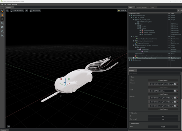
• Select the Streamlines_Volume_elements in the Stage panel.

• Navigate to the Property panel and locate the CaeAlgorithmsStreamlinesAPI section under Property.

• Next to Seeds, select Add Target and navigate to the UnitSphere created in the prior section (/CAE/UnitSphere).

• Next to Velocity, select Add Target and navigate to the velocity data (/Base/Volume/FlowSolution) and shift+select Velocity_m_s_0, Velocity_m_s_1, Velocity_m_s_2, hit select.

• To move the streamlines, select the UnitSphere and use the transform toggle to move the sphere. This updates the streamlines accordingly.

Note

Move the UnitSphere directly to update the streamlines, not the streamline prim directly.

• To color the streamlines by a scalar, under CaeAlgorithmsStreamlinesAPI, select Add Target next to Colors and select the desired scalar. Navigate to, and shift select FlowSolution/Velocity_m_s_0, Velocity_m_s_1 and Velocity_m_s_2.

• The color can be adjusted by changing the min and max values of the domain under Streamlines/Materials/ScalarColor/Shader.

Other important parameters in the Streamlines Properties:

Dx: step size between streamline vertex.

Max Length: The maximum distance the streamlines will be drawn.

Width: Width of the display of the streamlines.

Volume Render: IndeX (VTK based)

• Hide the Streamlines_Volume_elements created in the previous step (optional).

• Select Volume_elements node in the Stage panel. Right-click on the node to retrieve the context menu. Navigate to, and click on Create > CAE Algorithms > Volume (IndeX).

  • This creates another prim named /CAE/IndexVolume_Volume_elements.

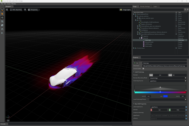
• In the newly created prim IndexVolume_Volume_elements go to Property, select Add Target next to Field and navigate to the flow results (/Base/Volume/FlowSolution) and select the velocity components.

The visual display can be adjusted via the Colormap under CAE/NanoVdbIndeXVolume_Volume_elements/Material/Colormap.

Create Flow Visualization

• Right-click on the kitCAE_Sample to retrieve the context menu. Navigate to, and click on Create > CAE Flow > Environment.

  • This creates another prim named /CAE/FlowEnvironment.

• Right-click on the node to retrieve the context menu and navigate to and click on Create > CAE Flow > DataSet Emitter.

  • This creates another prim named /CAE/DataSetEmitter_Volume_elements.

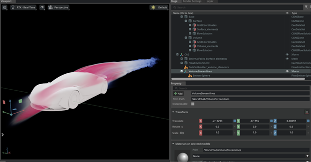
• Right-click on the node to retrieve the context menu and navigate to and click on Create > CAE Flow > VolumeStreamlines.

  • This creates another prim named /CAE/VolumeStreamlines.

• In /CAE/DataSetEmitter_Volume_elements navigate to Data.

• Next to Temperature > Add Target, navigate to, and select Wall_Shear_Stress_N_m2_mag.

• Next to Velocity > Add Target, navigate to, and select Velocity_m_s_0, Velocity_m_s_1, Velocity_m_s_2.

• Expand VolumeStreamlines and select EmitterSphere.

• Navigate to Property > Radius and change the radius to 0.5.

• Select VolumeStreamlines and move the Sphere in front of the vehicle.

• On the menu on the left, hit the play button. An animation will be shown.

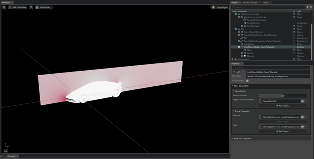
Create Slice Planes

• Hide the Flow Visualized created in the previous step, but keep the car surface displayed.

• In Stage/World/kitCAE_Sample_cgns/Base/Volume, right-click on the Volume_elements node to open the context menu. Navigate to, and click on Create > CAE Algorithms > Slice (IndeX).

  • This creates another prim named /CAE/IndeXSlice_Volume_elements.

• In /CAE/IndeXSlice_Volume_elements navigate to Slice (Unstructured), and then Field, and select Add Target.

• Navigate to, and select pressure from kitCAE_Sample_cgnsBaseVolumeFlowSolution.

• In /CAE/IndeXSlice_Volume_elements navigate to Extra Properties, find Field, and then select Add Target.

• Navigate to, and select velocity from kitCAE_Sample_cgnsBaseVolumeFlowNumPyArrays.

• Expand /CAE/IndeXSlice_Volume_elements. Select Plane, translate over desired slice region.

Note

The initial placement of the slice plane can be away from the region of interest, therefore, fit to screen (F on keyboard) and use the move toggle to adjust the placement into view.