Joint Parameter Tuning Example: Robotiq 2F-85#

Introduction#

The purpose of this document is to provide an example of tuning physics parameters for articulation joints, specifically joint drives, in the context of robotic gripper assets. The focus will be on joint drives based on a spring/damper model. This tuning example is geared towards using PhysX as the simulation backend, however, some of the recommendations likely apply to other simulators too. The robot gripper chosen for this tuning example is the Robotiq 2F-85 gripper.

Please note that this document is not intended as a comprehensive tuning guide. Corresponding information is available already (see the Links section). This document simply demonstrates an application of some of that knowledge. Additionally, there are some helper tools available, such as the gain tuner extension (see the Links section).

Caveats#

Note that all the parameter estimation helpers used in this document are very crude. They are not intended to provide precise results but to get a rough understanding of the value range from which to choose your parameters. With that in mind, a value of 10 m/s² will be used for gravity in all computations.

Links#

Preparation Work#

When tuning something like a gripper, it is often helpful to first create a set of very simple scenes that only contain the gripper (or just the hand part for a full humanoid robot) and one object to grasp. One testing sequence could involve starting with an open gripper and placing the object to grip between the pincers or fingers. Begin with gravity disabled on the object to grip. Let the gripper close around the object and observe for any instabilities or penetration. Once the gripping action reaches a steady state, enable gravity on the gripped object and check again for instabilities, penetration and whether the gripper can maintain its grip in the presence of gravity. An additional force can be applied on the grasped object to emulate a lifting movement.

For scene setup, the following scenarios are usually beneficial:

For the object to grasp, choose a primitive shape, such as a box or cylinder. Use 2-3 versions of this object to check the gripper’s behavior at different levels of closing. For example, use a thick box so that the gripper is almost fully open when gripping, a thin box so that the gripper is nearly fully closed, and a third setup where the gripper is somewhere between fully open and fully closed when gripping.
For the object to grasp, choose a shape that is challenging with respect to collision response and prone to penetration. For example, an object with thin walls like a cup or a bowl.
For the object to grasp, choose the geometrically most difficult one that the gripper will need to handle in your target application.

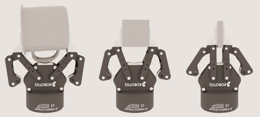
../../_images/gripper_test_scenarios.jpg — Figure 8 Example scenarios for testing the gripper.#

Robotiq 2F-85#

The gripper chosen for this example is the Robotiq 2F-85. The joints relevant to this exercise are shown in the image below.

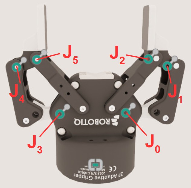
../../_images/gripper_joints_numbered.jpg — Figure 9 Joint setup for the Robotiq 2F-85.#

Six revolute joints were used to model the degrees of freedom of the gripper. It is a simplified version that does not use loop-closing joints. Joint J₀ is the only joint with a drive. The other five joints are all mimic joints of joint J₀ and are driven indirectly through that joint. The gearing value for all mimic joints is 1 (or -1), and the offset is 0. Joint J₀ has a motion range from 0 to 47 degrees, with 0 degrees resulting in the gripper being fully open and 47 degrees resulting in the gripper being fully closed.

Maximum Drive Force / Maximum Joint Velocity#

It is usually a good first step to set the limits on the drive forces and joint velocities. This ensures the simulation stays within a range that is expected for the real gripper. The corresponding numbers and information can typically be found in the mechanical specifications of the robot. If not, the manufacturer may need to be contacted to obtain the details. Another option is to gather the data by conducting experiments and measurements on the real robot.

Maximum Drive Force#

The Robotiq gripper has a useful example in the specifications, stating that it can hold a 5 kg box, assuming a friction coefficient of 0.3. Let’s use that setup and estimate how it translates to the joint drive at J₀. Holding 5 kg with a friction coefficient of 0.3 requires a force of roughly

(1)#\[\frac{mass \cdot gravity}{0.3} = \frac{5 \; kg \cdot 10 \; m/s^2}{0.3} \approx 166 \; N\]

That is the sum of the forces from both gripper fingers, so the force per finger is 83 N. However, we need to determine the torque at the joint, not the force at the contact point. The relationship between torque and force is given by:

(2)#\[\tau = F \cdot r\]

To calculate the torque \(\tau\), the “lever arm” r must be estimated. By examining the dimensions of the link that contains the finger pads, a rough estimate can be made. We will use a value of 0.04 m. As a result, the torque will be:

(3)#\[\tau = F \cdot r = 83 \; N \cdot 0.04 \; m \approx 3.3 \; Nm\]

Let’s round the value up and use 4 Nm to allow for a bit of a margin. Note that the link containing the finger pad is not directly connected to joint J₀, which has the drive. However, all the joints are connected via a mimic to the driven joint J₀, and as such, all joints are considered to be driven here. Furthermore, the gearing ratio for all mimic joints is 1. Thus, we can make the generous assumption that each joint will experience the same torque from the drive. To summarize, the estimated torque of 4 Nm is considered to be the maximum drive force for each joint.

One last important consideration before using this value to set the maximum drive force on joint J₀: the estimated torque is per joint, but joint J₀ has to drive all six joints (itself plus the five mimic joints). Consequently, the maximum drive force on joint J₀ is set to:

(4)#\[J_0 \; maxDriveForce = 6 \cdot 4 \; Nm = 24 \; Nm\]

Maximum Joint Velocity#

The Robotiq specification defines the maximum finger speed as 0.15 m/s. Let’s assume this speed can be maintained constantly from the gripper being fully open to fully closed. The distance between the fingers of the fully opened gripper is 0.085 m. Therefore, one finger needs to move 0.0425 m to close.

What does this mean for the angular velocity at joint J₀? Using a rough approximation, the time it takes for the gripper to close at maximum speed can be used to estimate the maximum angular velocity at joint J₀.

(5)#\[time \; to \; close \; gripper = t = \frac{distance}{maxSpeed} = \frac{0.0425 \; m}{0.15 \; m/s} \approx 0.28 \; s\]

As mentioned in a previous section, the joint position of J₀ ranges from 0 to 47 degrees to move from fully open to fully closed.

(6)#\[J_0 \; maxJointVelocity = \frac{angleTravelRange}{t} = \frac{47 \; deg}{0.28 \; s} \approx 168 \; deg/s\]

IMPORTANT: PhysX uses radians for maximum joint velocity, while USD is using degrees. The units must be mapped accordingly.

IMPORTANT: It is generally better not to set the maximum joint velocity on mimic joints (leaving them at the default maximum). Especially when using non-compliant mimic joints, instabilities could occur in certain cases if the maximum joint velocity on the mimic joints is set too low. Note that this is not a real limitation: if the joint being mimicked has a maximum joint velocity (like joint J₀ in our example), then the mimic joint should, by design, mimic that maximum velocity as well (considering the gearing ratio).

Drive Stiffness/Damping#

Joint drives using a spring/damper model generate a force of the form:

(7)#\[F = (s \cdot dx) - (d \cdot dv)\]

s: stiffness
d: damping
dx: delta between current position and target position
dv: delta between current velocity and target velocity

When choosing stiffness and damping values, it is often advisable to compute the natural frequency and the damping ratio (see the links provided in the Links section) of the spring/damper to check if the chosen simulation frequency is appropriate. Since the example gripper here uses revolute joints, the formulas are:

(8)#\[natural \; frequency = nf = \sqrt{\frac{s}{i}}\]

(9)#\[damping \; ratio = dr = \frac{d}{2 \cdot \sqrt{s \cdot i}}\]

i: inertia (for joints with a linear degree of freedom it would be mass instead)

Note that the natural frequency presented here is the natural angular frequency in radians per second. To get oscillations per second, the value would need to be divided by \(2 \pi\). This document will stick to natural angular frequency as it leads to a simpler rule of thumb in subsequent statements.

The Robotiq gripper simulation model in this example has only a single joint with a drive, J₀. However, the mimic joints get driven indirectly, so theoretically, all of them should be considered. Among this set of joints, the one that will lead to the most conservative values is the joint that connects to the link with the smallest inertia (or mass in the case of a joint with a linear degree of freedom). It is prudent to be on the conservative side for the following computations. Joint J₀ will be used here. The inertia around the rotation axis of the lighter link on J₀ is 2.1e-6 kg m². This value refers to the center of mass of the link. The joint, however, connects to the link at one end, not at the center of mass. The parallel axis theorem can be used to compute the inertia around a shifted rotation axis:

(10)#\[i^* = i + (m \cdot delta^2)\]

m: mass

delta: distance between shifted rotation axis and center of mass

The mass of the link in question is 0.0127 kg, and a delta 0.01 m will be used. This gives an adjusted inertia of:

(11)#\[2.1e\text{-}6 \; kg \; m^2 + (0.0127 \; kg \cdot (0.01 \; m)^2) \approx 3.4e\text{-}6 \; kg \; m^2\]

In absolute terms, this did not make much difference, but in relative terms, it did. Since everything here is just a rough approximation, it might not be worth making this extra correction, but for this exercise, the adjusted inertia value will be used.

The asset in its original form had a joint drive stiffness of about 5700 kg m²/s². Computing the natural frequency for this gives:

(12)#\[nf = \sqrt{\frac{5700 \; kg \; m^2/s^2}{3.4e\text{-}6 \; kg \; m^2}} \approx 4.0e4 \; rad/s\]

The asset was then simulated with a simulation time step that maps to a simulation frequency of 250 s^-1. Ideally, the simulation frequency should be somewhat close to the natural frequency. This is not the case here, as the natural frequency is much larger. When using the TGS solver, a larger number of position iterations allow for larger time steps (up to a certain point), but this is usually not proportional to the number of position iterations. Even with an over-optimistic assumption that 64 position iterations each count as full simulation steps, giving a simulation frequency of approximately 1.6e4 s^-1 (64 \(\cdot\) 250 s^-1), it is still quite a bit below the natural frequency of 4.0e4 rad/s. Such a setup is prone to cause problems.

Assuming it is not an option to increase the simulation frequency to be closer to the natural frequency, the latter must be reduced. Looking at the formula, the natural frequency can only be reduced by either decreasing the stiffness or increasing the inertia (or mass for a joint with a linear degree of freedom). For a specific robot, the inertia is usually a given (note that an inertia can be assigned to joints as well; see the section Armature), so decreasing stiffness is the only option. Given the simulation timestep size and as such the simulation frequency, one option could be to set the natural frequency equal to the simulation frequency and then compute the resulting stiffness.

(13)#\[s = nf^2 \cdot i\]

However, we will take a different approach here. Ultimately, the stiffness needs to be large enough to achieve the maximum drive force at a certain positional target delta. In the drive force formula, the stiffness-related force term was defined as:

(14)#\[F = s \cdot dx\]

This means the smaller the distance to the drive target, the smaller the force. Let’s assume the maximum drive force should be achieved until the delta to the target gets down to 0.005 m (e.g., gripping a box that is 0.01 m thick). Running the simulation shows that a target delta of 0.005 m at the finger corresponds to a joint position of roughly 42 degrees at joint J₀. To fully close the gripper, the angle must reach 47 degrees, so the target delta at joint J₀ is 5 degrees, or approximately 0.087 radians. The maximum drive force has been computed in a previous section, and now the target delta is known, so using (14), the matching stiffness can be computed.

(15)#\[s = \frac{F}{dx} = \frac{maxDriveForce}{0.087 \; rad} = \frac{24 \; Nm}{0.087 \; rad} \approx 275 \; kg \; m^2/s^2\]

Using this stiffness value to compute the natural frequency once more gives something in the order of 9.0e3 rad/s. While that is still significantly larger than the 250 s^-1 simulation frequency, it is clearly smaller than the over-optimistic 1.6e4 s^-1 simulation frequency (counting the 64 position iterations as full simulation steps). At this point, it seems worth trying to run with this setup and see if there are any simulation artifacts. During fine-tuning, it will likely make sense to try and lower the stiffness further (while ensuring that the maximum drive force can still be reached at the 0.087 radians target delta). It is important to state once more that very rough estimates are applied here, and one cannot expect precise outcomes. However, comparing the original stiffness of 5700 kg m²/s² to the newly computed value of 275 kg m²/s² shows how these estimates help to guide the value range to operate in.

Deriving the damping parameter is usually an easier task. Starting from the damping ratio, the damping parameter can be derived as follows:

(16)#\[d = dr \cdot 2 \cdot \sqrt{s \cdot i}\]

The damping ratio, dr, is usually an easier parameter to reason about than the damping parameter, d. A damping ratio of 1 means critical damping, where the target position should be reached without overshooting. Lower values than 1 mean there will be some oscillation around the target position before it is reached (and zero means no damping at all). Values larger than 1 will make movements more sluggish. A value of 1 is usually a good starting point unless there is clear knowledge that the robot joints require significant damping. Applying this to the Robotiq gripper with the previously computed stiffness:

(17)#\[d = 1.0 \cdot 2 \cdot \sqrt{275 \; kg \; m^2/s^2 \cdot 3.4e\text{-}6 \; kg \; m^2} \approx 0.06 \; kg \; m^2/s\]

IMPORTANT: PhysX and USD use different units for stiffness and damping. One unit of stiffness/damping in USD is equivalent to \(\frac{180}{\pi}\) units of stiffness/damping in PhysX. The units must be mapped accordingly. This document always uses the PhysX units, which are also the more commonly used units in general.

Implicit Spring#

PhysX uses an implicit formulation to compute the force of the spring/damper joint drive. The advantage of this approach is that it prevents excessively large forces from being created, even if users choose an inappropriately large timestep relative to the natural frequency of the joint drive. This makes the simulation less prone to instability and reduces the likelihood of it “exploding”. One might say this is achieved by adding some extra high damping. The downside is that it can result in unintuitive behavior. For example, increasing stiffness beyond a certain point will not result in the drive providing more force; instead, the drive will provide less force. Similarly, increasing damping beyond a certain point will lead to almost no damping force being applied. This is another reason to ensure that the natural frequency of joint drives is somewhat close to the chosen simulation frequency.

For the interested: why does increasing stiffness not provide more force at some point? Ignoring damping for now, the implicit spring force can be roughly described as:

(18)#\[F = \frac{s \cdot dx}{dt^2 \cdot nf^2 + 1}\]

The numerator \((s \cdot dx)\) matches the explicit spring force that has been discussed already. However, there is also a denominator. The interesting part of the denominator is:

(19)#\[dt^2 \cdot nf^2\]

If that part is close to zero, the implicit spring force will be the same as the explicit spring force. The larger this product gets, the smaller the spring force will be compared to the explicit version. This product will only be small if the timestep dt is small enough relative to the natural frequency nf. This is another example of the connection between simulation frequency and natural frequency.

Armature#

An inertia (or mass in the case of a joint with a linear degree of freedom) can be assigned to joints. This is called armature, named after the rotating coils in an electric motor. From a real robot perspective, this can describe the inertia/mass of a motor and/or a gearing system of the joint. From a tuning perspective, it is also a way to reduce the natural frequency of a joint drive. To reiterate some insight from a previous section: natural frequency is lowered by either decreasing stiffness or increasing inertia. It should be noted that this changes the physical setup of the joint, so it should be used with care. Unfortunately, relatively large values are often required to see an effect. As an exercise, a somewhat extreme case of using a large relative armature will be explored here, and the effect on the natural frequency will be shown. Let’s assume 5.0e-3 kg m² will be used. This will be added to the 3.4e-6 kg m² inertia that has been used for joint J₀ so far. Since 3.4e-6 is insignificant compared to 5.0e-3, let’s just use the latter as inertia. Computing the natural frequency then gives 234 rad/s (\(\sqrt{275 / 5.0e\text{-}3}\)). This is a lot lower than the previous value of 9.0e3 rad/s and suggests that it could work with a simulation frequency of 60 s^-1 (with the TGS solver and 64 position iterations). Actually testing this setup in one test scene indicated that it might indeed work without creating significant instability.

The benefits of armature make it an important paramter to setup properly. Electric-motor datasheets state the motor’s rotor inertia and can be used to compute the armature simulation parameter from the formula for reflected inertia at the gearbox output shaft of the electric drive system:

(20)#\[armature = i_m \cdot G^2\]

i_m: inertia of the motor rotor

G: ratio of motor angular velocity divided by the output shaft angular velocity

The armature of 5.0e-3 kg m² used in the earlier analysis may appear unrealistic when compared to the joint inertia of 3.4e-6 kg m² for joint J₀. However, assuming a gear ratio G of 50, we arrive at a motor rotor inertia of 2.0e-6 kg m² (5.0e-3 / 50²) that is the same order of magnitude as the joint inertia. Please note that the assumed gear ratio of 50 is not a real world estimate for the motors involved in the gripper used in this document. The value was simply chosen to demonstrate that large relative armature values might be applicable if the motor datasheet justifies such a choice.

To summarize: armature allows you to account for joint inertia that is otherwise not properly modeled. Depending on the specification of a joint motor, it can have a substantial impact on simulation behavior and reduces the natural frequency of a spring drive. When using armature values that are an order of magnitude larger than the inertia of the lighter joint link, it is advisable to double-check whether the motor specification and gear ratio actually support such a choice (otherwise, the physical properties might be modified to a degree that poorly reflects the real gripper). Lastly, increasing armature has its limits. At some point, it can also make the simulation behavior worse.

Mimic Joint Compliance#

Mimic joints try to keep the position and velocity of two joints in sync. They can either be configured as hard constraints, potentially creating large forces to prevent divergence between the two joints, or they can be configured as soft constraints (compliance) that “connect” two joints via a spring/damper model, which might allow for some divergence without immediately generating large forces. When tuning parameters on a gripper, it might be worth initially trying non-compliant mimic joints and only adding compliance once it becomes clear that too many hard constraints are fighting each other and cannot be resolved without the mimic joint yielding. Sometimes increasing armature (see the section Armature) can help resolve instabilities without having to resort to compliance. Note that, unlike joint drives, compliance on mimic joints is not set via stiffness and damping parameters. Instead, natural frequency and damping ratio must be set (see the section Drive Stiffness/Damping for details).

Compliant joints do not always steadily resolve divergence between joints as the natural frequency increases. When compliant mimic joints fight against hard constraints, it might seem as though the mimic joint is doing nothing at all. However, it might be that the mimic joint is simply too weak and is overruled by some hard constraint. Only above a certain natural frequency might the mimic joint show a significant effect in such a situation. That transition can be quite abrupt.

IMPORTANT: Having read this document up to this point and managed to stay awake, it should be clear that natural frequency is not stiffness, and that damping ratio is not damping (the parameters are just related). Nevertheless, it has been observed more than once that users pick the stiffness and damping values from a joint drive and copy them into the natural frequency and damping ratio parameters of a mimic joint. That is incorrect, and hopefully, this document made it clear why.

Verification and Fine-Tuning#

Once all the relevant parameters have been roughly tuned, it is time to verify the effects and do some fine-tuning. It is recommended to perform verification on a set of simple scenes first (see the section Preparation Work). These scenes should verify that:

The simulation roughly reflects the maximum gripper speed specified (e.g., by checking how long it takes for the simulation to go from fully open gripper to fully closed and comparing that with the information from the official robot specification).
The gripper can hold the maximum load under gravity as defined in the robot specification (when friction coefficients, etc., match). This should be tested for various gripper finger states (from almost fully open to almost fully closed, or as closed as the value used to compute the stiffness, assuming the approach in this documentation is used. See the section Drive Stiffness/Damping, which chose a 0.01 m gap as the smallest delta to reach maximum drive force).
There is no significant penetration. Note that visual meshes can sometimes be misleading. For example, a cup might have thinner walls on the visual mesh than on the simulation collision object. It is helpful to visualize the collision object via debug properties in omni.physx or use a physics recording tool like OVD to see in detail what was happening in the simulation.
There is no significant jitter or other instabilities.

These simple scenes are also a good playground to fine-tune physics parameters. For example, can stiffness and/or maximum joint drive force be reduced on joints while still being able to hold the maximum load? If yes, then it might make sense to rather use the lower values. If values are adjusted, do not forget to also adjust other related parameters. For example, when changing the stiffness, it should be considered to also re-compute the damping parameter. If penetration, jitter or other instabilities are still observed despite having based all the parameters on the robot specification and the proposed estimation schemes in this document, it might be time to try increasing the position iteration count, decreasing the timestep size (increase the simulation frequency), or adding/increasing armature on the joints.

There is little value in starting to simulate a whole humanoid and interaction with more complex objects/environments until the gripper or hand behaves as expected in all the simple scenes. Another advantage of testing with simple scenes is that they are much faster to re-run repeatedly, and they are also easier to debug and analyze.