Rigid-Body Simulation

Rigid bodies and static colliders are the building blocks that you can use to add physics to your scene. You can add rigid body dynamics to a geometry in your scene so that it accelerates under gravity and collides with other physics objects (including deformables and fluid), and create static physics objects by adding collision to scene geometry (e.g. a basic ground plane).

For further, in-depth technical detail on the rigid-body simulation standard in USD, you may refer to the UsdPhysics Schema Doc.

Adding Dynamics to a Geometry

Any prim that has a transform can be made into a rigid body (i.e. any USD Xformable-derived prim). Examples include geometric shapes like Cube or Sphere, or Mesh prims. Adding rigid-body simulation to a prim is straightforward: Either right-click the prim in the viewport or stage tree, or use the Add Button in the prim’s property window, and do Add > Physics > Rigid Body with Colliders Preset.

The name of the preset highlights the two main components that a dynamic rigid body typically has:

1. A rigid body component which provides dynamics-related properties such as linear and angular velocity, or whether the body is kinematic.

2. a collision component which is applied to body geometry that defines the collision-shape which determines how the body collides with other collision-enabled objects on the stage (e.g. a ground plane or a deformable body), and provides related properties, see Collision Settings.

You may configure the rigid-body and collision parameters in the corresponding rollouts in the Property Window. For details on the parameters, refer to the tool tips.

The typical USD and physics component structure that you encounter when you turn assets into rigid-bodies is that of a compound-shape rigid body.

Static Colliders

If you apply only the collision component to an asset with Add > Physics > Colliders Preset, you create a Static Collider. Static colliders do not move (unless you move them) but still collide with other Physics objects (e.g. rigid or deformable bodies). Therefore, this is the configuration you should choose, for example, for the floor and walls of a physics-enabled room scene. A very simple static collider is the Physics ground plane that you can add to a scene with Create > Physics > Ground Plane.

Note that the Colliders Preset traverses all descendants of the target prim and applies a separate collider component to every suitable descendant so that assets consisting of multiple meshes become a single compound static collider. Of course, you can apply the component to specific meshes of an asset as well: Just use Add > Physics > Collider on the target meshes.

Compound-Shape Rigid Bodies and USD Hierarchy

Typically, graphics assets consist of several meshes that should move together. The Rigid Body with Colliders Preset provides automation to achieve this when you apply it to the common (USD-hierarchy) parent of the meshes that should move together. Let us look at an example of two barstools falling onto static-collider cubes:

The right stool is a compound rigid body, while the left stool is four separate rigid bodies corresponding to each of the meshes of the asset. In the USD stage, the compound stool’s structure and component-assignments are as follows:

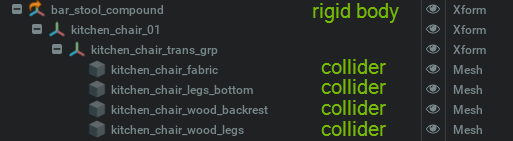
I.e. the preset applied the rigid body component to the parent Xform and then traversed all the descendants of the Xform while applying the Colliders Preset to any geometry it encountered. The result is the compound stool.

For the left stool, we applied the preset to each of the four meshes, so there is no rigid-body component on the parent Xform, but each collider component also has a rigid-body component in addition.

In the video, you may have noticed that the collision of the stool’s legs with the cubes are not reflecting the actual geometry of the legs. This is due to the default convex-hull collision-geometry approximation that the preset applies. See Collision Settings for further information and a video of the stools with improved collision approximation.

A compound-structure with just a single collision geometry can also be useful to create a rigid body that has separate collision and visualization geometries. A simple example is:

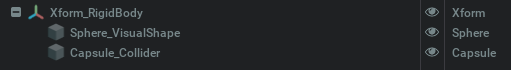
The rigid-body component is applied to the parent Xform, the sphere shape serves as visualization, and the capsule provides the collision geometry. The capsule is excluded from rendering by setting the render Purpose to guide in the Visual property-window rollout. A possible intent is to make the sphere roll along a straight line more easily; in more complex, Mesh-based geometry applications you can use this approach to fine-tune the collision geometry of a high-detail visual mesh.

Note

• You cannot nest rigid bodies - any rigid-body component found among the USD-hierarchy descendants of a prim with a rigid-body component is ignored. Except if that descendant’s transform op stack has a resetXformStack op.

• You may animate, i.e. change the relative transforms of the nested collision geometries making up the rigid body, which updates the inertial properties of the compound rigid body. However, such an animation does not impart momentum onto the compound; if that is your intent, you should use Articulations or separate rigid bodies with Joints instead.

Kinematic Rigid Bodies

The rigid-body rollout provides a checkbox to make the rigid body kinematic. The resulting simulation object is similar to a static collider: It only moves if you change its transform through the UI, or through a script or animation. However, the advantage of using a kinematic body for animation is that the simulation infers a continuous velocity for the body from the transforms (i.e. keyframes) that you provide, and this velocity is imparted to dynamic bodies during collisions, which results in higher simulation fidelity.

Another way to think about dynamic vs. kinematic rigid bodies is in terms of transform read/write access by the simulation engine: A dynamic body has its transform written to by the simulation, while a kinematic rigid body’s transform is read by the simulation (static colliders are also read-only).

Instancing Rigid Bodies

There are two approaches to increasing performance when dealing with many identical rigid bodies (or colliders) in a scene: USD Scenegraph Instancing and the USD Point Instancer. Both reduce the size of the USD scene graph which in turn increases performance and reduces the scene’s memory footprint.

Instancing

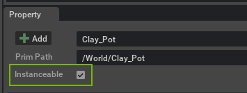
When you drag-and-drop an asset from the Content Window into the stage, you are creating a reference to the asset. If you require many copies of the asset in your scene, it is best to turn the references into instances. You can achieve this by enabling the Instanceable flag in the property window:

Instancing is straightforward if you are creating duplicates of static colliders, but for rigid bodies there is an important consideration: The Rigid Body component must be added to each instance and not the referenced asset (i.e. master/prototype). The reason for this is that the rigid-body component provides properties that describe the state of the object (e.g. its linear velocity) which are unique for each instance, and, therefore, the instances cannot share a single rigid-body component on the referenced asset. A typical rigid-body instancing setup would be as follows:

1. Add the collider component to the source asset (considering the limitations on mesh-approximations for rigid bodies)

2. Create a reference to the asset using drag-and-drop from the content window

3. Enable the Instanceable flag on the reference

4. Add the Rigid Body component to the reference (you do not need the preset that also applies the collider, as the source asset already provides it to all instances)

5. Create duplicates of the instanceable rigid body

If you create instances of a static collider, you can skip the rigid-body-component-adding step.

Point Instancer

An alternative approach is the USD Point Instancer feature. Currently, you can only create a point instancer via the Python API, so you best refer to the Instanced box on a plane snippet source code in the physics demo scenes for more information. The advantage of the point instancer is that it provides a vectorized interface to the poses and velocities of the instances.

Mass Properties

By default, the mass of a dynamic rigid body is derived from the volume of its collision geometry, multiplied by a density. For compounds, the mass is the sum of the masses of its collision geometries, see below. Unless a density is specified explicitly, a default of 1000 kg/m³ is used (scaled to scene units).

One can set an explicit density in two ways: 1) By binding a physics material to the collision geometry, or 2) by adding a Mass component (Add > Physics > Mass) to the collision geometry or a rigid-body ancestor. A density specified in a Mass component overrides any material density.

You can also use the Mass component to set the mass of a collision geometry directly. An explicit mass overrides any densities specified on the geometry. In summary, the precedence is:

Default 1000kg/m³ < Material density < Mass-component density < Mass-component mass

Note that if there is no collision geometry to derive mass via density, the mass defaults to 1.0 mass units.

Local-space velocities

It is possible to set and output velocities for a rigid body in local space, it can be enabled in the properties window.

• For angular velocity, the velocity is transformed by the rigid body world rotation.

• For linear velocity, the velocity is transformed by the rigid body world rotation and its scale.

Compounds and USD Hierarchy

For compounds, you can specify mass properties for each of the collision geometries following the precedence rule above. A collision geometry of a compound may inherit an explicit density set on an ancestor, so there are additional USD-hierarchical precedence rules:

• Ancestors’ mass properties override descendants’ properties according to the precedence rule above.

• For equal-level precedence, e.g. Mass-component density, the descendants specific values override the ancestor specifications.

This is not straightforward to parse, so we illustrate it further with the barstool example in the Compounds Section: We can add a Mass component to the stool rigid-body Xform and set a homogeneous density (e.g. the density of wood): The stool mass is then equal to the sum of the collision-geometry volumes times this explicit density.

Alternatively, we could model the stool’s mass more accurately by considering the fabric seat’s lower density. We apply a Mass component to the fabric seat and set it to the lower density. The stool parts without a density specified then use the overall (wood) density while the seat uses the lower density when the overall mass is computed.

If in addition, we specify a mass with the Mass component on the stool rigid-body Xform, all the densities we set earlier are ignored due to the precedent rule and the stool’s specified mass is homogeneously distributed among the collision geometry meshes.

Collision Settings

Collisions enable rigid bodies to interact with each other and a static-collider environment. The key parameters that determine collision behavior are:

• How the geometry of the object is approximated for the PhysX engine

• Physics Material Properties such as friction and restitution (bounciness)

• PhysX collision parameters such as, for example, collision and rest offset

Rigid-Body Collision Mesh Approximation

For dynamic rigid bodies, PhysX currently does not support using the asset (triangle) mesh directly for collision. The mesh geometry must be approximated with one of the following methods available in the Collider rollout of the property window:

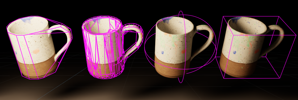
The pink lines represent the Collider debug visualization that is useful for analyzing the generated approximations. From left to right are:

1. Convex Hull: PhysX computes a convex hull for the asset mesh. If you require a tighter approximation or representing concave features, choose a Convex Decomposition instead.

2. Convex Decomposition: PhysX performs a convex decomposition where the input mesh is approximated by several convex shapes. This allows approximating hollow meshes such as the cup above.

3. A bounding sphere.

4. A bounding box.

5. A SDF (signed distance filed) approximation.

Note

• For both convex approximations, the vertex count per convex shape is limited to 60 for GPU acceleration support.

• SDF colliders are described in their own section sdf collision

Static-Collider Collision Mesh Approximation

In addition to the rigid-body approximation methods, static colliders support triangle-mesh collision. Often, you can reduce the mesh complexity without losing much detail by selecting the mesh simplification option, see the right simplified cup mesh vs. the original on the left:

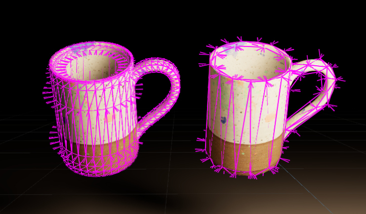
Note the short lines sticking out from the collider debug visualization mesh are the normals, which allow you to determine the orientation of the mesh faces, see note below.

Note

• Physics treats meshes as single sided for collision purposes, i.e. collisions only occur with the meshes’ front. In contrast, Omniverse renders all meshes as double-sided by default. This discrepancy may result in a scene that has unexpected collision behavior while rendering fine. We recommend that in the Rendering > Render Settings window, under the Common tab, users authoring physics colliders enable Geometry > Back Face Culling so it becomes clear which faces are front versus back facing.

• If a mesh has faces facing the wrong way, they can be inverted using the Geometry > Orientation dropdown in the Property window of the mesh.

• You can inspect the normals drawn onto the collider debug visualization to determine the orientation (see the cups’ triangle-mesh debug visualization above).

Barstools Revisited

In the barstool example above, the collision geometry is not well captured by the default convex-hull approximation and the hollow space between the legs collides with the cube. We can fix this by changing the collision approximation of the leg meshes to convex decomposition. The resulting collision is more accurate:

Note that changing the collision approximation and the associated geometry may impact the rigid body’s mass distribution if mass properties are computed from the collision geometry (e.g. by a specified density).

Shapes

PhysX supports exact representations for Cube, Capsule, and Sphere shapes, so no approximations are required. By default, the Cone and Cylinder shapes are approximated with a convex hull. However, PhysX supports exact representation of the Cone and Cylinder as well if you enable the Custom Geometry flag in their Collider settings. Note that enabling the Custom Geometry flag currently incurs a performance penalty in a (by default) GPU simulation because part of the collision code runs on the CPU. Also note that Custom Geometry is CPU-only yet, and therefore cannot interact with GPU-only features such as soft bodies or particles.

Parameters

Besides the Collider properties, collision parameters are available in the Physics Material of the collision shape. For further details on the parameters, we refer to their Tool Tips. The offset parameters are explained in more detail below:

The Collision Offset defines a small distance from the surface of the collision geometry at which contacts start being generated. The default value is -inf which means that the application tries to determine a suitable value based on scene gravity, simulation frame rate and object size. Increase this parameter if fast-moving objects are missing collisions, i.e. tunnel (alternatively, check Enable CCD in the rigid body and the PhysicsScene for swept contact detection). Increasing the offset too much incurs a performance penalty since more contacts are generated between objects that need to be processed at each simulation step.

The Rest Offset defines a small distance from the surface of the collision geometry at which the effective contact with the shape takes place. It can be both positive and negative, and may be useful in cases where the visualization mesh is slightly smaller than the collision geometry: setting an appropriate negative rest offset results in the contact occurring at the visually correct distance.

Collider Compatibility

PhysX does not yet support collisions between all collision geometry. In particular, the GPU-only features, for example Particles, are not compatible with CPU-only colliders such as the Custom Geometry Cone and Cylinder, for example. We summarize the compatibility in the table below.

Collider Compatibility Table

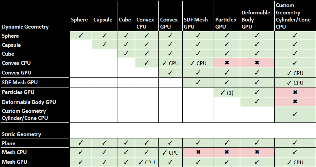
Table Notes

• ✓ CPU: compatible, running on CPU. See also performance consideration notes below.

• ✓ (1): Particles can collide within the same particle system, but cannot collide with particles that are in another particle system.

Geometry Notes

• Sphere: includes Mesh Bounding Sphere, and Sphere Approximation

• Cube: includes Mesh Bounding Cube

• Convex CPU: Convex Hulls are cooked for both CPU and GPU compatibility in general and automatically use the appropriate data and compute device depending on the simulation running on CPU or GPU. A CPU-only convex is generated if the input mesh data (before scaling) is oblong, in which case you will get a warning in the console: [Warning] [omni.physx.cooking.plugin] ConvexMeshCookingTask: failed to cook GPU-compatible mesh, collision detection will fall back to CPU. Collisions with particles and deformables will not work with this mesh. Prim /World/Cone

• Mesh CPU: Triangle meshes are cooked for both CPU and GPU compatibility in general and automatically use the appropriate data and compute device depending on the simulation running on CPU or GPU. A multi-material triangle mesh is a CPU-only mesh.

Performance Considerations with CPU Geometry

In general, CPU collision geometry generates contacts on the CPU, while GPU collision geometry generates contacts on the GPU. Most geometry supports both CPU and GPU, e.g. Spheres or Convex Hulls (see note above), and automatically uses the appropriate compute device based on the simulation running on the CPU or on the GPU.

GPU-only collision geometry such as Deformable Bodies or Particles can only be used when GPU simulation is enabled. However, this is not true for some of the CPU-only collision geometry with GPU simulation: For example, the Custom Geometry Cone can collide with a dynamic SDF Mesh. This is achieved by running the contact generation on CPU, which may incur a performance penalty that you may want to be aware of for large GPU simulations, for example a reinforcement learning setup. In the table above, CPU/GPU collision pairs that are supported but run on the CPU are marked accordingly (✓ CPU).

PhysX SDF Collision

The Signed-Distance-Field (SDF) collision detection feature allows the simulation of dynamic and kinematic rigid bodies that use high-detail triangle meshes as their collision shape. Demos like Nuts and Bolts and Chair Stacking leverage the SDF feature to simulate the contact-rich interaction between dynamic objects of highly non-convex shape. SDFs can help to speed up collision detection between dynamic triangle meshes a lot and are a requirement for triangle mesh colliders on dynamic objects.

The SDF is computed by PhysX on a uniform grid with a grid spacing equal to the mesh’s longest AABB extent divided by an SDF Resolution attribute, see instructions below. Sparse SDFs are supported and recommended to reduce the amount of memory required to store the distance field.

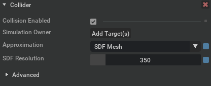
How to Enable SDF Collision

In the collision mesh Collider rollout, set the Approximation to SDF Mesh and set a nonzero SDF Resolution. SDFs use quite a bit of memory but help to accelerate the collision detection a lot. To reduce the memory consumption, it is recommended to use sparse SDFs where a lot of distance samples are stored near the triangle mesh’s surface but fewer samples further away from the surface. Additionally, quantization of the distance values should be activated for sparse SDFs since this allows to further reduce the memory consumption while still being accurate enough in almost all cases. Quantization can be controlled by adjusting the SDF Bits per Subgrid Pixel in the Advanced section. Sparse SDFs and quantization are enabled by default. Dense SDFs are still available by setting the SDF Subgrid Resolution to zero in the Advanced section.

When you change the SDF resolution or start the simulation, PhysX will cook the SDF data which can take a couple of seconds up to a couple minutes for very high SDF resolutions combined with a complex mesh. It is not recommended to use exceedingly high resolutions, as it will waste resources. In most cases, resolutions of 250 already produce good results, resolutions higher than 1000 are very rarely used. It is usually better to split the mesh into multiple smaller parts when working with SDFs on big objects.

Best Practices and Debugging

If the collision response is not satisfactory, it is recommended to check the following settings. Not all of them are directly related to SDFs but they all influence the collision behavior.

• Increase the maximal number of contacts per frame

  • In complex scenes, it is possible that a lot of contacts get generated, especially by SDF colliders. In some cases the default value for the maximal number of contacts that can be processed per frame might be too low. If the collision response seems to be incorrect, it is worth to try increasing the maximal number of Gpu contacts in the Physics Scene. If there is not Physics Scene in the Stage, one can be added using Create/Physics/Physics Scene. The relevant options to increase the number of contacts that can be stored are in the Physics Scene Api’s Gpu rollout and are called “Gpu Max Rigid Contact Count” and “Gpu Max Rigid Patch Count”. Usually doubling the values until the collision artifacts are gone is a good strategy. For smaller scenes, the default values should be large enough.

• Adjust the SDF resolution

  • A too low SDF resolution can lead to situations where very thin parts of the mesh don’t collide since the SDF cannot represent/capture them

  • A too high SDF resolution might lead to increased memory consumption and a bit slower collision detection performance

• Use meshes with a good tessellation when generating the SDF

  • Watertight triangle meshes without self intersections or other defects simplify the cooking process. In case the mesh has holes, the cooker closes them but the closing surface will be defined by the cooker

• Increase the contact offset

  • Larger contact offsets allow the solver to react a bit earlier to collisions potentially happening in subsequent timesteps. Too large contact offsets will slow down the collision detection performance, so it’s usually an iterative process of finding a good value

• Make objects heavier, within reasonable limits

  • Objects that are extremely lightweight or if objects with very different mass come in contact, the collision response might not be perfect since those cases make convergence of the solver more difficult

• Reduce the maximal depenetration velocity

  • Makes the collision response a bit slower and can help to avoid overshooting

• Increase the number of position iterations

  • Gives the solver more iterations to improve convergence

• Increase friction

  • Helps that objects in contact come to rest

• Reduce the timestep of the physics simulation

  • This is only recommended if all other adjustments don’t lead to good results

Debug Visualization and Pre-Computation

You may inspect the generated SDF using debug visualization available in the Physics Debug Window:

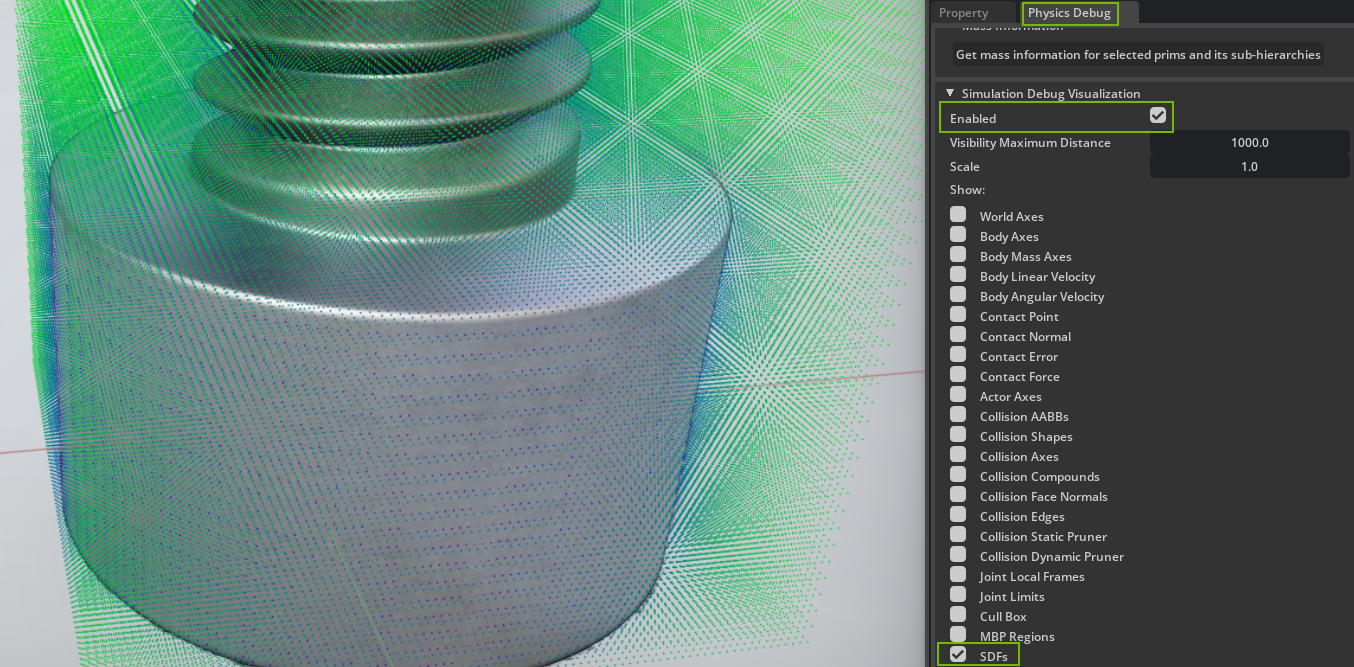
After cooking, the generated SDF is stored into a cooked data API, so a subsequent simulation starts up faster, and you can save individual assets with their SDF data pre-computed (which is used in the demos to speedup startup time).

Note

• Multi-material triangle-mesh colliders are not supported with the SDF collision feature.

• For more details, see the paper Factory: Fast Contact for Robotic Assembly

Rigid-Body Materials

Rigid-body physics materials provide friction, restitution (a.k.a. ‘bounciness’), and material density properties. See the precedence rules in Instancing Rigid Bodies for density defined via materials. Static collider’s meshes support multiple materials by assigning materials to geometry subsets; see the Triangle Mesh Multimaterial snippet in the physics demo scenes for more information.

If a rigid body or static collider does not have an assigned material, a default material is applied with dynamic friction = static friction = restitution = 0.5. You may change the default material properties by binding a physics material to the Physics Scene. See also the Physics Material section for general physics material information.

Collision Filtering

The Physics extension supports collision filtering that you can use to disable collision between pairs and groups of physics objects (including rigid and deformable bodies, and articulations).

Collision Groups

You can create Collision Groups that are sets of colliders. The groups can be configured to enable or disable collisions between them.

Create a new group with Create > Physics > Collision Group. Then you can add colliders to its Includes and Excludes relationships, subject to inheritance rules defined by the Expansion Rule.

All objects in the same collision group collide with each other. By default, objects in two different collision groups also collide, but you can disable collisions between groups by adding to their Filtered Groups relationship. The PhysicsScene provides a flag Invert Collision Group Filter that lets you invert this behavior so that by default, different groups do not collide, except for Filtered Groups-specified collisions.

Note

• Currently, collision groups cannot be changed during simulation and require stopping and restarting the simulation. This will be addressed in a future release.

Pairwise Collision Filter

In cases where using collision groups is insufficiently fine grained, one may select two bodies, colliders or articulations, and choose Add > Physics > Pair Collision Filter. This disables collision between the selected objects and their property windows have a Filtered Pairs rollout added. Pairwise filters have precedence over collision groups.

Note

• Currently, pair filtering cannot be changed during simulation and requires stopping and restarting the simulation. This will be addressed in a future release.

Joints

Joints give you the ability to connect physics objects by defining how the objects may move relative to each other. For example, a revolute joint can be used to connect a wheel to a car’s chassis: It allows the wheel to rotate around a single axis.

Joints may create connections between all types of rigid objects, i.e. dynamic and kinematic rigid bodies, static colliders, and also Articulations (i.e. their rigid-body links in particular). It is also possible to connect objects to the static world coordinate frame if you leave one of the joint’s Body relationships empty (which is then implicitly relating to the world frame).

In the overview table about joint types, you also find information about what joints can be simulated natively by Articulations and are compatible with, i.e. can create connections to articulation links.

Debug Visualization of the joints not only displays the joints and their frames, but allows authoring of the joint frames as well - just enable Joints in the Debug Visualization viewport options.

For joints tutorial please watch this video: Rigging a Desk Lamp

Types

Explore the different joint motions with the Physics Demo Snippets that are available for each of the joint types.

Type	Description	Articulations native compatible
	The revolute joint allows rotation about a single axis.	yes yes
	The prismatic joint allows linear motion along a single axis.	yes yes
	The spherical joint allows rotation about three axes, i.e. a ball-in-socket-type joint.	yes yes
	The D6 joint can be configured to allow between zero and six degrees of relative motion, i.e. up to three linear plus three rotational motions. Use Joint Limits to lock individual axes. Articulations can natively simulate D6 joints with 1-3 unlocked rotational motions (all linear motion must be locked).	(yes) yes
	The fixed joint allows no relative motion. It is particularly useful when building fixed-base Articulations.	yes yes
	The distance joint allows any relative motion but limits how far apart the connected rigid bodies may be (in particular their joint frames).	no yes
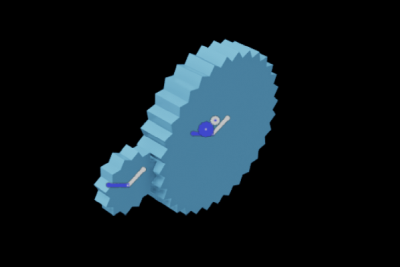
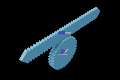
	The gear joint couples the rotations of two revolute joints by a gear ratio. See the snippet and its Python code for details.	no yes
	The rack-and-pinion joint couples the rotation of a revolute joint to the travel of a prismatic joint by a gear ratio (rotation/distance). See the snippet and its Python code for details.	no yes

Joint Frames

Each of the two physics objects that are connected by a joint has an associated joint frame. The joint frame is fixed and positioned in the body’s local frame using the Local Position 0/1 and Local Rotation 0/1 properties.

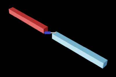
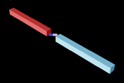
Any joint motion is relative to the bodies’ configuration where the two joint frames are aligned: For example, a revolute joint configured to rotate around the x-axis allows rotation of the two body frames about their shared x axis, and at zero joint angle, the two frames are aligned. An offset is illustrated in the following revolute joint example:

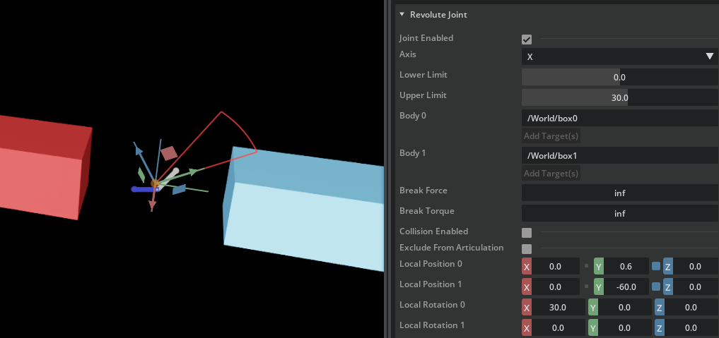
The revolute joint connects the red and blue geometries that are configured as a static collider (red) and dynamic rigid body (blue) respectively. Let us focus on the Local Rotations first. The Local Rotation 0 for box0 is thirty degrees around x which is reflected in the joint-frame visualization. As soon as the simulation is started, the blue box will rotate up to align its frame (that is not rotated). The thirty degree Joint Limit is relative to the aligned frames as well (see the see red lines and arc visualization).

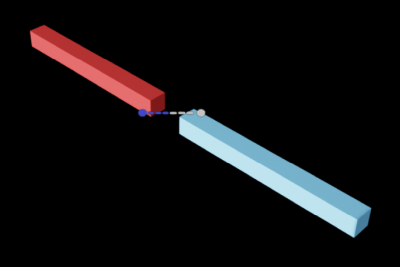
In the same example, you will notice the different values used to define the (y) local positions of the frames: 0.6 and -60.0. The reason is that joint positions scale together with a body. In the example, the red box0 is created from a unit-cube with side-length 1.0 which is then scaled by 10.0, 100.0, 10.0 in x, y, and z, respectively. The blue box1 is created from a cube with side-length 100.0 which is scaled by 0.1, 1.0, 0.1 in x, y, and z, respectively. Therefore, both geometries have the same world dimensions, but their different scaling results in the joint frames being correctly positioned by the 0.6 (times 100.0) and -60 in y, respectively.

Joint Limits

Some joints provide limit properties directly in their corresponding rollout, so you can configure ranges for the relative motion that the joints allow (e.g. thirty degrees rotation in the revolute joint example above).

For the D6 joints, you can add limit components in order to lock or limit specific axes with Add > Physics > Limit in the D6’s property window. In order to lock an axis, set the lower limit to above the high limit. See the D6 Joint snippet in the demo scenes as well.

Note

• Due to differences in the underlying PhysX implementation, spherical joint limits are pyramidal in native articulation joints, and conical for regular spherical joints.

• Revolute joints with limits are simulated using PhysX SDK unwrapped revolute joints, which enables setting drive targets and joint limits outside the regular revolute joint angle wrap at +/- 2pi. The revolute joint type is determined at simulation start, and enabling/disabling limits later on cannot change the type.

Joint Drives

Many joints support adding drives so you can physically actuate a mechanism (vs. kinematic animation). For example, you can add a drive to a revolute joint that connects a wheel to a car to make it move. Add the drive with Add > Physics > (type) Drive where the type will be context-sensitive and describing the motion of the drive (e.g. angular for a revolute joint).

Drives apply a force to the joint to maintain a position and/or a velocity that is proportional to

stiffness * (position - target_position) + damping * (velocity - target_velocity)

so the stiffer you configure the drive, the harder it will push the bodies to satisfy a given target position for the drive. Damping is analogous for the joint velocity, and you can implement a velocity drive by setting stiffness to zero.

Note

Spherical joints currently do not support drives, but you may configure a D6 joint with drives to get the same driven motion, including native simulation support in articulations.

RigidBody xformOp reset and sanitation

Simulation output cant write to arbitrary xformOp order stack. Therefore we do sanitation of the xformOp stack to work with simulation.

These steps happen when play is pressed:

• RigidBody xformOp stack is stored with xformOp attributes and values

• If the xformOp stack is translate, orient, scale nothing happens, if other stack is found its cleared and replaced by translate, orient, scale stack.

• Simulation writes output into translate and orient (quaternion).

• When simulation ends, xformOp stack is replaced with the stored xformOp attributes from simulation start.